Phylogenetic Comparative Methods learning from trees
- Chapter 9: Beyond the Mk Model
- Section 9.1: The Evolution of Frog Life History Strategies
- Section 9.2: Beyond the Mk model
- Section 9.3: Pagel’s λ, δ, and κ (lambda, delta, and kappa)
- Section 9.4: Mk models where parameters vary across clades and/or through time
- Section 9.5: Threshold models
- Section 9.6: Modeling more than one discrete character at a time
- Section 9.7: Testing for non-independent evolution of different characters
- Section 9.8: Chapter summary
R markdown to recreate analyses
Chapter 9: Beyond the Mk Model
Section 9.1: The Evolution of Frog Life History Strategies
Frog reproduction is one of the most bizarrely interesting topics in all of biology. Across the nearly 6,000 species of living frogs, one can observe a bewildering variety of reproductive strategies and modes (Zamudio et al. 2016). As children, we learn of the “classic” frog life history strategy: the female lays jellied eggs in water, which hatch into tadpoles, then later metamorphose into their adult form [e.g. Rey (2007); Figure 9.1A]. But this is really just the tip of the frog reproduction iceberg. Many species have direct development, where the tadpole stage is skipped and tiny froglets hatch from eggs. There are foam-nesting frogs, which hang their eggs from leaves in foamy sacs over streams; when the eggs hatch, they drop into the water [e.g. Fukuyama (1991); Figure 9.1B]. Male midwife toads carry fertilized eggs on their backs until they are ready to hatch, at which point they wade into water and their tadpoles wriggle free [Marquez and Verrell (1991); Figure 9.1C]. Perhaps most bizarre of all are the gastric-brooding frogs, now thought to be extinct. In this species, female frogs swallow their fertilized eggs, which hatch and undergo early development in their mother’s stomach (Tyler and Carter 1981). The young were then regurgitated to start their independent lives.
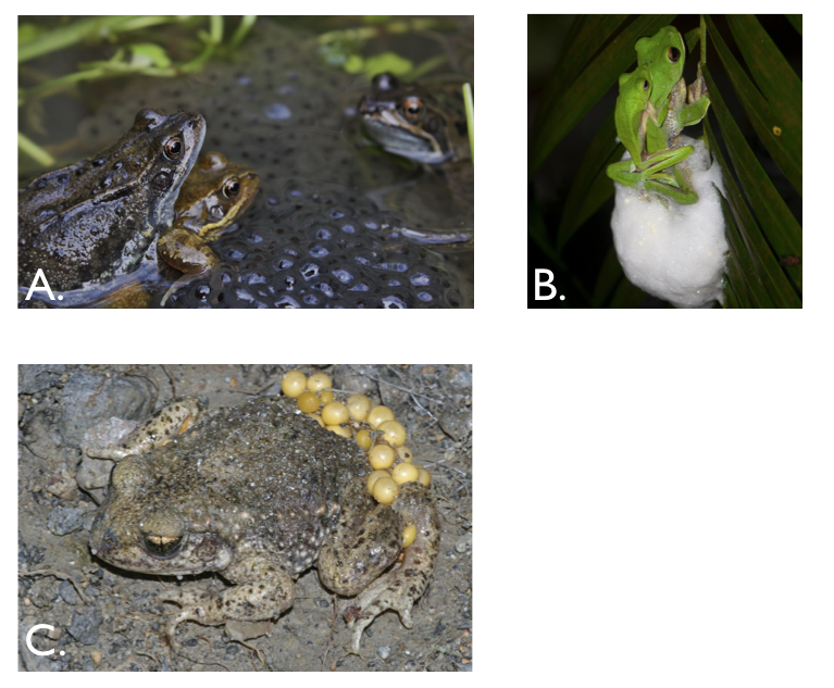
Figure 9.1. Examples of frog reproductive modes. (A) European common frogs lay jellied eggs in water, which hatch as tadpoles and metamorphose; (B) Malabar gliding frogs make nests that, supported by foam created during amplexus, hang from leaves and branches; (C) Male midwife toads carry fertilized eggs on their back. Photo credits: A: Thomas Brown / Wikimedia Commons / CC-BY-2.0, B: Vikram Gupchup / Wikimedia Commons / CC-BY-SA-4.0 C: Christian Fischer / Wikimedia Commons / CC-BY-SA-3.0
The great diversity of frog reproductive modes brings up several key questions that can potentially be addressed via comparative methods. How rapidly do these different types of reproductive modes evolve? Do they evolve more than once on the tree? Were “ancient” frogs more flexible in their reproductive mode than more recent species? Do some clades of frog show more flexibility in reproductive mode than others?
Many of the key questions stated above do not fall neatly into the Mk or extended-Mk framework presented in the previous characters. In this chapter, I will review approaches that elaborate on this framework and allow scientists to address a broader range of questions about the evolution of discrete traits.
To explore these questions, I will refer to a dataset of frog reproductive modes from Gomez-Mestre et al. (2012), specifically data classifying species as those that lay eggs in water, lay eggs on land without direct development (terrestrial), and species with direct development (Figure 9.2).
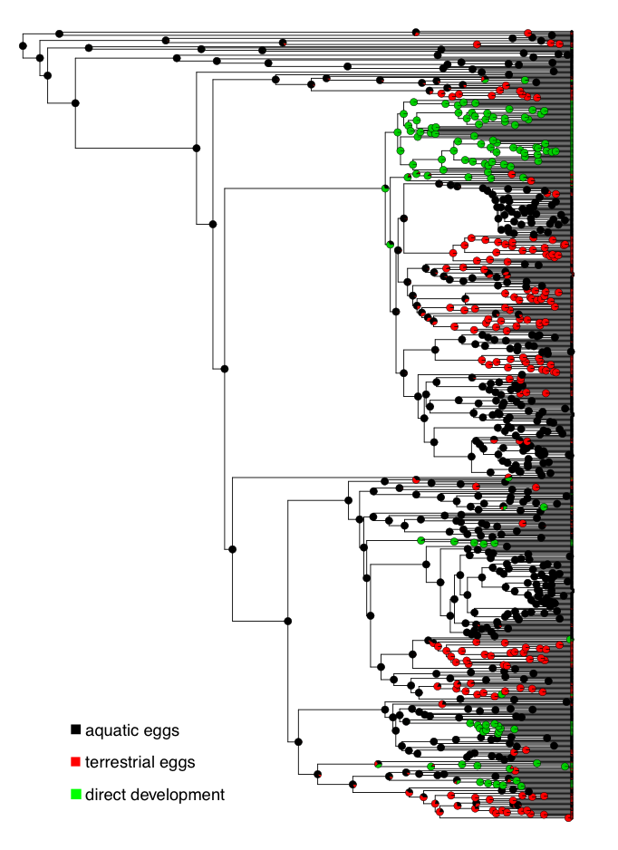
Figure 9.2. Ancestral state reconstruction of frog reproductive modes. Data from Gomez-Mestre et al. (2012). Image by the author, can be reused under a CC-BY-4.0 license.
Section 9.2: Beyond the Mk model
In Chapter 8, we considered the evolution of discrete characters on phylogenetic trees. These models fall under the general category of continuous-time Markov models, which consider a process that can occupy two or more states. Transitions occur between those states in continuous time. The Markov property means that, at some time t, what happens next in the model depends only on the current state of the process and not on anything that came before.
In evolutionary biology, the most detailed work on continuous time Markov models has focused on DNA or protein sequence data. As mentioned earlier, an extremely large set of models are available for modeling and analyzing these molecular sequences. One can also elaborate on these models by adding rate heterogeneity across sites (e.g. the gamma parameter, as in GTR + Γ), or other complications related to mechanisms of sequence evolution (for a review, see Liò and Goldman 1998).
However, there are two important differences between models of sequence evolution and models of character change on trees that make our task distinct from the task of modeling DNA or amino acid sequences. First, when analyzing molecular sequences, one typically has data for many thousands (or millions) of characters. Data sets for other characters – like the phenotypic characters of species – are typically much smaller (and harder to collect). Second, sequence analysis very often assumes that each character evolves independently from all other characters, but that all characters (or at least certain large subsets of those characters) evolve under a shared model (Liò and Goldman 1998; Yang 2006). This means that, for example, the frequency of transitions between A and C at one location in a gene sequence contribute information about the same transition in a different location in the sequence.
Unfortunately, when analyzing morphological character evolution, we are often interested in single characters, and the use of shared models across characters seems impossible to justify. There is usually no equivalence between different character states for different characters: an A is an A for sequences, but a “1” in a character matrix usually corresponds to the presence of two completely different characters. The consequence of this difference is reflected in the statistical property of multivariate data. For gene sequence problems, adding more data in the form of additional characters (sites) makes model-fitting easier, as each site adds information about the overall (shared) model across sites. With character data, additional characters do not make the problem any easier, because each character comes with its own model parameters. In fact, we will see that when considering character correlations using a generalized Mk model, adding characters actually makes the problem more and more difficult. Perhaps these issues partially explain the slow pace of model development for fitting discrete characters to trees. There are a few potential solutions, such as threshold models [Felsenstein (2005); Felsenstein (2012); discussed below]. More work is desperately needed in this area.
In this chapter, we will first discuss extensions of Mk models that allow us to add complexity to this simple model. We also discuss threshold models, a relatively new approach in comparative methods that is distinct from Mk models and has some potential for future development.
Section 9.3: Pagel’s λ, δ, and κ (lambda, delta, and kappa)
The three Pagel models discussed in chapter 6 (Pagel 1999a,b) can also be applied to discrete characters. We do not create a phylogenetic variance-covariance matrix for species under an Mk model, so these three models can, in this case, only be interpreted in terms of transformations of the tree’s branch lengths. However, the meaning of each parameter is the same as in the continuous case: λ scales the tree from its original form to a “star” phylogeny, and thus quantifies whether the data fits a tree-based model or one where all species are independent; δ captures changes in the rate of trait evolution through time; and κ scales branch lengths between their original values and one, and mimics a speciational model of evolution (but only if all species are sampled and there has been no extinction).
Just as with discrete characters, the three Pagel models can be evaluated in either an ML / AICc framework or using Bayesian analysis. One might expect these models to behave differently when applied to discrete rather than continuous characters, though. The main reason for this is that discrete characters, when they evolve rapidly, lose historical information surprisingly quickly. That means that models with high rates of character transitions will be quite similar to both models with low “phylogenetic signal” (i.e. λ = 0) and with rates that accelerate through time (i.e. δ > 0). This indicates potential problems with model identifiability, and warns us that we might not have good power to differentiate one model from another.
We can apply these three models to data on frog reproductive modes. But first, we should try the Mk and extended-Mk models. Doing so, we find the following results:
| Model | lnL | AICc | ΔAICc | AIC Weight |
|---|---|---|---|---|
| ER | -316.0 | 633.9 | 38.0 | 0.00 |
| SYM | -296.6 | 599.2 | 3.2 | 0.17 |
| ARD | -291.9 | 596.0 | 0.0 | 0.83 |
We can interpret this as strong evidence against the ER model, with ARD as the best, and weak support in favor of ARD over SYM. We can then try the three Pagel parameters. Since the support for SYM and ARD were similar, we will add the extra parameters to each of them. Doing so, we obtain:
| Model | Extra parameter | lnL | AICc | ΔAICc | AIC weight |
|---|---|---|---|---|---|
| ER | -316.0 | 633.9 | 38.0 | 0.00 | |
| SYM | -296.6 | 599.2 | 5.2 | 0.02 | |
| ARD | -291.9 | 596.0 | 0 | 0.37 | |
| SYM | λ | -296.6 | 601.2 | 5.2 | 0.02 |
| SYM | κ | -296.6 | 601.2 | 5.2 | 0.02 |
| SYM | δ | -295.6 | 599.2 | 3.2 | 0.07 |
| ARD | λ | -292.1 | 598.3 | 2.3 | 0.11 |
| ARD | κ | -291.3 | 596.9 | 0.9 | 0.24 |
| ARD | δ | -292.4 | 599.0 | 3.0 | 0.08 |
Notice that our results are somewhat ambiguous, with AIC weights spread fairly evenly across the three Pagel models. Interestingly, the overall lowest AIC score (and the most AIC weight, though only just more than 1/3 of the total) is on the ARD model with no additional Pagel parameters. I interpret this to mean that, for these data, the standard ARD model with no alterations is probably a reasonable fit to the data compared to the Pagel-style alternatives considered above, especially given the additional complexity of interpreting tree transformations in terms of evolutionary processes.
Section 9.4: Mk models where parameters vary across clades and/or through time
Another generalization of the Mk model we might imagine is a Mk model where rate parameters vary, either across clades or through time. There is some recent work along these lines, with two approaches that consider the possibility that rates of evolution for an Mk model vary on different branches of a phylogenetic tree (Marazzi et al. 2012; Beaulieu et al. 2013).
We can understand how these methods work in general terms by considering a simple case where the rate of character evolution is faster in one clade than in the rest of the tree. This is the discrete-character version of the approaches for continuous characters that I discussed in chapter 6 (O’Meara et al. 2006; Thomas et al. 2006). The simplest way to implement a multi-rate discrete model is to directly incorporate variation across models into the pruning algorithm that is used to calculate the Mk model on a phylogenetic tree (see FitzJohn 2012 for implementation).
One can, for example, consider a model where the overall rate of evolution varies between clades in a phylogenetic tree. To do this, we can specify the background rate of evolution using some transition matrix Q, and then assume that within our focal clade evolution can be modeled with some scalar value r, such that the new rate matrix is rQ. Given Q and r, one can calculate the likelihood for this model using the pruning algorithm, modified in such a way that the appropriate transition matrix is used along each branch in the tree; one can then maximize the likelihood of the model for all parameters (those describing Q, as well as r, which describes the relative rate of evolution in the focal clade compared to the background).
In even more general terms, we will consider the situation where we can describe the model of evolution using a set of Q matrices: Q1, Q2, …, Qn, each of which can be assigned to a particular branch in a phylogenetic tree (or be assigned to branches depending on some other character that influences the rate of the focal character; Marazzi et al. 2012). The only limit here is that each Q matrix adds a new set of model parameters that must be estimated from the data, and it is easy to imagine this model becoming overparametized. If we imagine a model where every branch has its own Q-matrix, then we are actually describing the “no common mechanism” model (Tuffley and Steel 1997; Steel and Penny 2000), which is statistically identical to parsimony. It should also be possible to create a method that explores all models connecting simple Mk and the no common mechanism model using the machinery of reversible-jump MCMC, although I do not think such an approach has ever been implemented (but see Huelsenbeck et al. 2004).
One can also describe a situation where rate parameters in the Q matrix change through time. This might follow a constant pattern of increase or decrease through time, or might be related to some external driver like temperature. One can mimic models where rates change through time by changing the branch lengths of phylogenetic trees. If deep branches are lengthened relative to shallow branches, as is done by Pagel's δ, then we can fit a model where rates of evolution slow through time; conversely, lengthening shallow branches relative to deep ones creates a model where the overall rate of evolution accelerates through time (see FitzJohn 2012).
More work could certainly be done in the area of time-varying rates of change. The most general approach is to write a set of differential equations that describe the changes in character state along single branches in the tree. Parameters in those equations can be made to vary, either through time or even in a way that is correlated with some external variable hypothesized to influence rates of change, like temperature or rainfall. Given such a model, the reverse-time approach of Maddison et al. (2007) can then be used to fit general time-varying (or even clade-varying) Mk models to data (see Uyeda et al. 2016).
Section 9.5: Threshold models
Recently, Joe Felsenstein (2005, 2012) introduced a model from quantitative genetics, the threshold model, to comparative methods. Threshold models work by modeling a discrete character as underlain by some other, unobserved, continuous trait (called the liability). If the liability crosses a certain threshold value, then the discrete state changes. More specifically, we can consider a single trait, y, with two states, 0 and 1, which is in turn determined by some underlying continuous variable, x, called the liability. If x is greater than the threshold, t, then y is 1; otherwise, y is 0. Felsenstein (2005) assumes that x evolves under a Brownian motion model, although other models like OU are, in principle, possible.
We can find the likelihood to this model by considering the observations of character states at the tips of the tree. We observe the state of each species, yi. We do not know the liability values for these species. However, we treat these liabilities as unobserved and consider their distributions. Under a Brownian motion model, we know that the liabilities will follow a multivariate normal distribution (see chapter 3). We can calculate the probability of observing the data (yi) by finding the integral of the distributions of liabilities on the side of the threshold that matches the data. So if the distribution of the liability for species i is pi(x), then:
(eq 9.1)
$$
p(y_i = 0) =
{\int\limits_{-\infty}^{t} p_i (x) dx}
$$
$$
p(y_i = 1) =
{\int\limits_{t}^{\infty} p_i (x) dx}
$$
(see Figure 9.3 for an illustration of this calculation, which is easier than it looks since there are standard formulas for finding the area under a normal distribution).
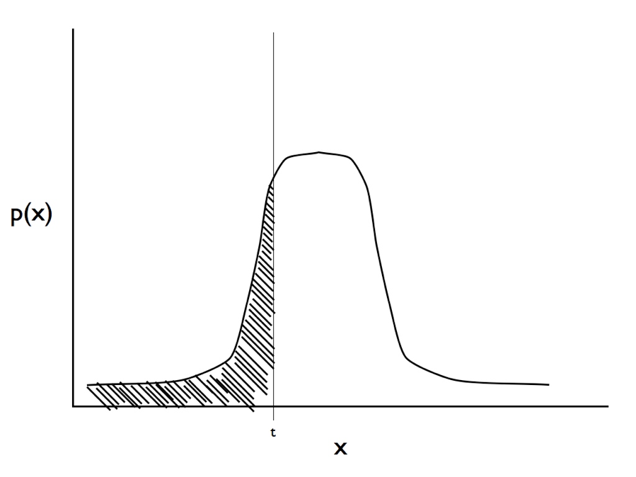
Figure 9.3. Illustration of the integral in equation 9.1. For a trait with observed state zero we calculate the area under the curve from negative infinity to the threshold t. Image by the author, can be reused under a CC-BY-4.0 license.
One can fit this model using standard ML or Bayesian methods. Current implementations include an expectation-maximization (EM) algorithm (Felsenstein 2005, 2012) and a Bayesian MCMC (Revell 2014).
The threshold model differs in some key ways from standard Mk-type models. First of all, threshold characters evolve differently than non-threshold characters because of their underlying liability. In particular, the effective rate of change of the discrete character depends on the amount of time that a lineage has been in that character state. Characters that have just changed (say, from 0 to 1) are likely to change back (from 1 to 0), since the liability is likely to be near the threshold. By contrast, characters that have been in one state or the other for a long time tend to be more unlikely to change (since the liability is likely very far from the threshold). This difference matches biological intuition for some characters, where millions of years in one state means that change to a different state might be unlikely. This behavior of the threshold model can potentially account for variation in transition rates across clades without adding additional model parameters. Second, the threshold model scales to cover more than one character more readily than Mk models. Finally, in a threshold framework, it is straightforward to extend the model to include a mixture of both discrete and continuous characters – basically, one assumes that the continuous characters are like “observed liabilities,” and can be modeled together with the discrete characters.
Section 9.6: Modeling more than one discrete character at a time
It is extremely common to have datasets with more than one discrete character – in fact, one could argue that multivariate discrete datasets are the cornerstone of systematics. Nowadays, the most common multivariate discrete datasets are composed of genetic/genomic data. However, the foundations of modern phylogenetic comparative biology were laid out by Hennig (1966) and the other early cladists, who worked out methods for using discrete character data to obtain phylogenetic trees that show the evolutionary history of clades.
Almost all phylogenetic reconstruction methods that use discrete characters as data make a key assumption: that each of these characters evolves independently from one another. Mathematically, one calculates the likelihood for each single character, then multiplies this likelihood (or, equivalently, adds the log-likelihood) across all characters to obtain the likelihood of the data.
The assumption of character independence is clearly not true in general. In the case of morphological characters, structures often interact with one another to determine the fitness of an individual, and it seems very likely that those structures are not independent. In fact, some times we are specifically interested in whether or not particular sets of characters evolve independently or not. Methods that assume character independence a priori are not useful for that sort of framework.
Felsenstein (1985) made a huge impact on the field of evolutionary biology with a statistical argument about species: species can not be considered independent data points because they share an evolutionary history. Species that are most closely related to one another will covary, simply due to that shared history. Nowadays, one cannot publish a paper in comparative biology without accounting directly for the non-independence of species that evolve on a tree. However, it is still very common to ignore the non-independence of characters, even when they occur together in the same organism! Surely the shared developmental history of two characters within one body commonly leads to correlations across these characters.
Section 9.7: Testing for non-independent evolution of different characters
Hypotheses in evolutionary biology often relate to whether two (or more) traits affect the evolution of one another (see Chapter 5). One can have a standard correlation between two discrete traits if knowing the state of one trait allows you to predict the state of the other. However, in evolution, these correlations will arise due to the shared patterns of relatedness across species. We are typically more interested in evolutionary correlations (see Chapter 5). With discrete traits, we can define evolutionary correlations in a specific way: two discrete traits share an evolutionary correlation if the state of one character affects the relative transition rates of a second.
Imagine that we are considering the evolution of two traits, trait 1 and trait 2, on a phylogenetic tree. Both traits have two possible character states, one and zero. We can show these two traits visually as Figure 9.4.
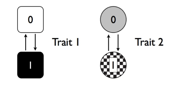
Figure 9.4. Two discrete character traits, each with two states (labeled 0 and 1). Image by the author, can be reused under a CC-BY-4.0 license.
In the figure, each trait has two possible transition rates, from 0 to 1 and from 1 to 0. For now, let’s assume that backwards and forward rates are equal. Any species can have one of four possible combinations of the two traits (00, 01, 10, or 11). We can draw the transitions among these four combinations as Figure 9.5.
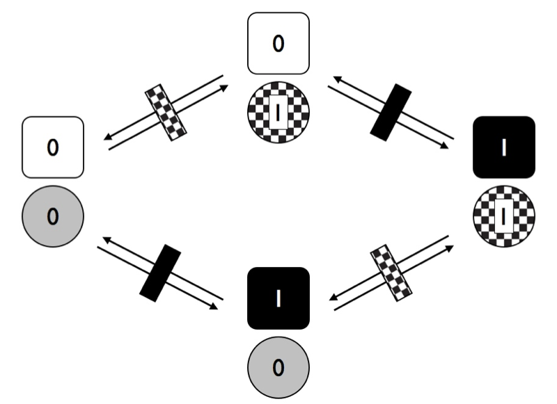
Figure 9.5. Transitions among states for two traits with two character states each where characters evolve independently of one another. Image by the author, can be reused under a CC-BY-4.0 license.
In Figure 9.6, I have marked the distinct rates with different rectangles – black represents changes in trait 1, while checkered is changes in trait 2. Notice that, in this figure, we are assuming that the two traits are independent. That is, in this model the transition rates of trait one do not depend on the state of trait 2, and vice-versa. What would happen to our model if we allow the traits to evolve in a dependent manner?
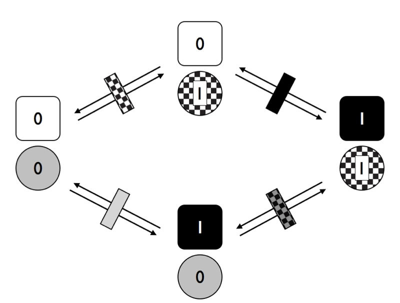
Figure 9.6. Transitions among states for two traits with two character states each where characters evolve at rates that depend on the character state of the other trait. Image by the author, can be reused under a CC-BY-4.0 license.
Notice that in Figure 9.6, we have four different transition rates. Consider first the solid rectangles. The grey rectangle represents the transition rate for trait 1 when trait 2 has state 0, while the black rectangle represents the transition rate for trait 1 when trait 2 has state 1. If these two rates are different, then the traits are dependent on each other – that is, the rate of evolution of trait 1 depends on the character state of trait 2.
These two models have different numbers of parameters, but are relatively easy to fit using the maximum-likelihood approach outlined in this chapter. The key is to write down the transition matrix (Q) for each model. For example, a transition matrix for model in figure 9.4 is:
(eq. 9.2)
$$
\mathbf{Q} =
\begin{bmatrix}
-q_1 - q_2 & q_1 & q_2 & 0\\
q_1 & -q_1 - q_2 & 0 & q_2\\
q_2 & 0 & -q_1 - q_2 & q_1\\
0 & q_2 & q_1 & -q_1 - q_2\\
\end{bmatrix}
$$
In the matrix above, each row and column corresponds to a particular combination of states for character 1 and 2: (0,0), (0,1), (1,0), and (1,1). Note that some possible transitions in this model have rate 0, meaning they do not occur. These are transitions that would require both characters to change exactly simultaneously (e.g. (0,0) to (1,1) – a possibility that is excluded from this model.
Similarly, we can write a transition matrix for the model in figure 9.5:
(eq. 9.3)
$$
\mathbf{Q} =
\begin{bmatrix}
-q_1 - q_2 & q_1 & q_2 & 0\\
q_1 & -q_1 - q_3 & 0 & q_3\\
q_2 & 0 & -q_2 - q_4 & q_4\\
0 & q_3 & q_4 & -q_3 - q_4\\
\end{bmatrix}
$$
Notice that the simple, 2-parameter independent evolution model is a special case of the more complex, 4-parameter dependent model. Because of this, we can compare the two with a likelihood ratio test. Alternatively, AIC or Bayes factors can be used. If we find support for the 4-parameter model, we can conclude that the evolution of at least one of the two characters depends on the state of the other.
It is worth noting that there are other models that one can fit for the evolution of two binary traits that I did not discuss above. For example, one can model the situation where the two traits each have different forwards and backwards rates, but are evolving independently. This is a four-parameter model. Additionally, one can allow both forward and backward rates to differ and to depend on the character state of the other trait: an eight-parameter model. This is the model one needs to truly see a correlation between the two characters, one where certain combinations tend to accumulate in the tree. All of these models – and others not described here – can be compared using AIC, BIC, or Bayes Factors. Pagel and Meade (2006) describe a particularly innovative and synthetic method to test hypotheses about correlated evolution of discrete characters in a Bayesian framework using reversible-jump MCMC.
One can also test for correlations among discrete characters using threshold models. Here, one tests whether or not the liabilities for the two characters evolve in a correlated fashion. More specifically, we can model liabilities for the two threshold characters using a bivariate Brownian motion model, with some evolutionary covariance σ122 between the two liabilities. We can then use either ML or Bayesian methods to determine if the evolutionary covariance between the two characters is non-zero (following the methods described in chapter 5, but using likelihoods based on discrete characters as described above).
Section 9.8: Chapter summary
The simple Mk model provides a useful foundation for a number of innovative methods. These methods capture evolutionary processes that are more complicated than the original model, including models that vary through time or across clades. Modeling more than one discrete character at a time allows us to test for the correlated evolution of discrete characters.
Taken as a whole, chapters 7 through 9 provide a basis for the analysis of discrete characters on trees. One can test a variety of biologically relevant hypotheses about how these characters have changed along the branches of the tree of life.
References
Beaulieu, J. M., B. C. O’Meara, and M. J. Donoghue. 2013. Identifying hidden rate changes in the evolution of a binary morphological character: The evolution of plant habit in campanulid angiosperms. Syst. Biol. 62:725–737.
Felsenstein, J. 2012. A comparative method for both discrete and continuous characters using the threshold model. Am. Nat. 179:145–156.
Felsenstein, J. 1985. Phylogenies and the comparative method. Am. Nat. 125:1–15.
Felsenstein, J. 2005. Using the quantitative genetic threshold model for inferences between and within species. Philos. Trans. R. Soc. Lond. B Biol. Sci. 360:1427–1434.
FitzJohn, R. G. 2012. Diversitree: Comparative phylogenetic analyses of diversification in R. Methods Ecol. Evol. 3:1084–1092.
Fukuyama, K. 1991. Spawning behaviour and male mating tactics of a foam-nesting treefrog, Rhacophorus schlegelii. Anim. Behav. 42:193–199. Elsevier.
Gomez-Mestre, I., R. A. Pyron, and J. J. Wiens. 2012. Phylogenetic analyses reveal unexpected patterns in the evolution of reproductive modes in frogs. Evolution 66:3687–3700.
Hennig, W. 1966. Phylogenetic systematics. University of Illinois Press.
Huelsenbeck, J. P., B. Larget, and M. E. Alfaro. 2004. Bayesian phylogenetic model selection using reversible jump markov chain monte carlo. Mol. Biol. Evol. 21:1123–1133.
Liò, P., and N. Goldman. 1998. Models of molecular evolution and phylogeny. Genome Res. 8:1233–1244.
Maddison, W. P., P. E. Midford, S. P. Otto, and T. Oakley. 2007. Estimating a binary character’s effect on speciation and extinction. Syst. Biol. 56:701–710. Oxford University Press.
Marazzi, B., C. Ané, M. F. Simon, A. Delgado-Salinas, M. Luckow, and M. J. Sanderson. 2012. Locating evolutionary precursors on a phylogenetic tree. Evolution 66:3918–3930.
Marquez, R., and P. Verrell. 1991. The courtship and mating of the Iberian midwife toad Alytes cisternasii (Amphibia: Anura: Discoglossidae). J. Zool. 225:125–139. Blackwell Publishing Ltd.
O’Meara, B. C., C. Ané, M. J. Sanderson, and P. C. Wainwright. 2006. Testing for different rates of continuous trait evolution using likelihood. Evolution 60:922–933.
Pagel, M. 1999a. Inferring the historical patterns of biological evolution. Nature 401:877–884.
Pagel, M. 1999b. The maximum likelihood approach to reconstructing ancestral character states of discrete characters on phylogenies. Syst. Biol. 48:612–622.
Pagel, M., and A. Meade. 2006. Bayesian analysis of correlated evolution of discrete characters by reversible-jump markov chain monte carlo. Am. Nat. 167:808–825.
Revell, L. J. 2014. Ancestral character estimation under the threshold model from quantitative genetics. Evolution 68:743–759.
Rey, H. A. 2007. Curious George: Tadpole trouble. Houghton Mifflin Harcourt.
Steel, M., and D. Penny. 2000. Parsimony, likelihood, and the role of models in molecular phylogenetics. Mol. Biol. Evol. 17:839–850.
Thomas, G. H., R. P. Freckleton, and T. Székely. 2006. Comparative analyses of the influence of developmental mode on phenotypic diversification rates in shorebirds. Proc. Biol. Sci. 273:1619–1624.
Tuffley, C., and M. Steel. 1997. Links between maximum likelihood and maximum parsimony under a simple model of site substitution. Bull. Math. Biol. 59:581–607.
Tyler, M. J., and D. B. Carter. 1981. Oral birth of the young of the gastric brooding frog rheobatrachus silus. Anim. Behav. 29:280–282. Elsevier.
Uyeda, J. C., L. J. Harmon, and C. E. Blank. 2016. A comprehensive study of cyanobacterial morphological and ecological evolutionary dynamics through deep geologic time. PLoS One 11:e0162539. Public Library of Science.
Yang, Z. 2006. Computational molecular evolution. Oxford University Press.
Zamudio, K. R., R. C. Bell, R. C. Nali, C. F. B. Haddad, and C. P. A. Prado. 2016. Polyandry, predation, and the evolution of frog reproductive modes. Am. Nat. 188 Suppl 1:S41–61.