Phylogenetic Comparative Methods learning from trees
- Chapter 3: Introduction to Brownian Motion
- Section 3.1: Introduction
- Section 3.2: Properties of Brownian Motion
- Section 3.3: Simple Quantitative Genetics Models for Brownian Motion
- Section 3.4: Brownian motion on a phylogenetic tree
- Section 3.5: Multivariate Brownian motion
- Section 3.6: Simulating Brownian motion on trees
- Section 3.7: Summary
- Footnotes
Chapter 3: Introduction to Brownian Motion
Section 3.1: Introduction
Squamates, the group that includes snakes and lizards, is exceptionally diverse. Since sharing a common ancestor between 150 and 210 million years ago (Hedges and Kumar 2009), squamates have diversified to include species that are very large and very small; herbivores and carnivores; species with legs and species that are legless. How did that diversity of species’ traits evolve? How did these characters first come to be, and how rapidly did they change to explain the diversity that we see on earth today? In this chapter, we will begin to discuss models for the evolution of species’ traits.
Imagine that you want to use statistical approaches to understand how traits change through time. To do that, you need to have an exact mathematical specification of how evolution takes place. Obviously there are a wide variety of models of trait evolution, from simple to complex. For example, you might create a model where a trait starts with a certain value and has some constant probability of changing in any unit of time. Alternatively, you might make a model that is more detailed and explicit, and considers a large set of individuals in a population. You could assign genotypes to each individual and allow the population to evolve through reproduction and natural selection.
In this chapter – and in comparative methods as a whole – the models we will consider will be much closer to the first of these two models. However, there are still important connections between these simple models and more realistic models of trait evolution (see chapter five).
In the next six chapters, I will discuss models for two different types of characters. In this chapter and chapters four, five, and six, I will consider traits that follow continuous distributions – that is, traits that can have real-numbered values. For example, body mass in kilograms is a continuous character. I will discuss the most commonly used model for these continuous characters, Brownian motion, in this chapter and the next, while chapter five covers analyses of multivariate Brownian motion. We will go beyond Brownian motion in chapter six. In chapter seven and the chapters that immediately follow, I will cover discrete characters, characters that can occupy one of a number of distinct character states (for example, species of squamates can either be legless or have legs).
Section 3.2: Properties of Brownian Motion
We can use Brownian motion to model the evolution of a continuously valued trait through time. Brownian motion is an example of a “random walk” model because the trait value changes randomly, in both direction and distance, over any time interval. The statistical process of Brownian motion was originally invented to describe the motion of particles suspended in a fluid. To me this is a bit hard to picture, but the logic applies equally well to the movement of a large ball over a crowd in a stadium. When the ball is over the crowd, people push on it from many directions. The sum of these many small forces determine the movement of the ball. Again, the movement of the ball can be modeled using Brownian motion1.
The core idea of this example is that the motion of the object is due to the sum of a large number of very small, random forces. This idea is a key part of biological models of evolution under Brownian motion. It is worth mentioning that even though Brownian motion involves change that has a strong random component, it is incorrect to equate Brownian motion models with models of pure genetic drift (as explained in more detail below).
Brownian motion is a popular model in comparative biology because it captures the way traits might evolve under a reasonably wide range of scenarios. However, perhaps the main reason for the dominance of Brownian motion as a model is that it has some very convenient statistical properties that allow relatively simple analyses and calculations on trees. I will use some simple simulations to show how the Brownian motion model behaves. I will then list the three critical statistical properties of Brownian motion, and explain how we can use these properties to apply Brownian motion models to phylogenetic comparative trees.
When we model evolution using Brownian motion, we are typically discussing the dynamics of the mean character value, which we will denote as $\bar{z}$, in a population. That is, we imagine that you can measure a sample of the individuals in a population and estimate the mean average trait value. We will denote the mean trait value at some time t as $\bar{z}(t)$. We can model the mean trait value through time with a Brownian motion process.
Brownian motion models can be completely described by two parameters. The first is the starting value of the population mean trait, $\bar{z}(0)$. This is the mean trait value that is seen in the ancestral population at the start of the simulation, before any trait change occurs. The second parameter of Brownian motion is the evolutionary rate parameter, σ2. This parameter determines how fast traits will randomly walk through time.
At the core of Brownian motion is the normal distribution. You might know that a normal distribution can be described by two parameters, the mean and variance. Under Brownian motion, changes in trait values over any interval of time are always drawn from a normal distribution with mean 0 and variance proportional to the product of the rate of evolution and the length of time (variance = σ2t). As I will show later, we can simulate change under Brownian motion model by drawing from normal distributions. Another way to say this more simply is that we can always describe how much change to expect under Brownian motion using normal distributions. These normal distributions for expected changes have a mean of zero and get wider as the time interval we consider gets longer.
A few simulations will illustrate the behavior of Brownian motion. Figure 3.1 shows sets of Brownian motion run over three different time periods (t = 100, 500, and 1000) with the same starting value $\bar{z}(0) = 0$ and rate parameter σ2 = 1. Each panel of the figure shows 100 simulations of the process over that time period. You can see that the tip values look like normal distributions. Furthermore, the variance among separate runs of the process increases linearly with time. This variance among runs is greatest over the longest time intervals. It is this variance, the variation among many independent runs of the same evolutionary process, that we will consider throughout the next section.
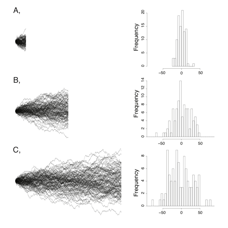
Figure 3.1. Examples of Brownian motion. Each plot shows 100 replicates of simulated Brownian motion with a common starting value and the same rate parameter σ2 = 1. Simulations were run for three different times: (A) 10, (B) 50, and (C) 100 time units. The right-hand column shows a histogram of the distribution of ending values for each set of 100 simulations. Image by the author, can be reused under a CC-BY-4.0 license.
Imagine that we run a Brownian motion process over a given time interval many times, and save the trait values at the end of each of these simulations. We can then create a statistical distribution of these character states. It might not be obvious from figure 3.1, but the distributions of possible character states at any time point in a Brownian walk is normal. This is illustrated in figure 3.2, which shows the distribution of traits from 100,000 simulations with σ2 = 1 and t = 100. The tip characters from all of these simulations follow a normal distribution with mean equal to the starting value, $\bar{z}(0) = 0$, and a variance of σ2t = 100.
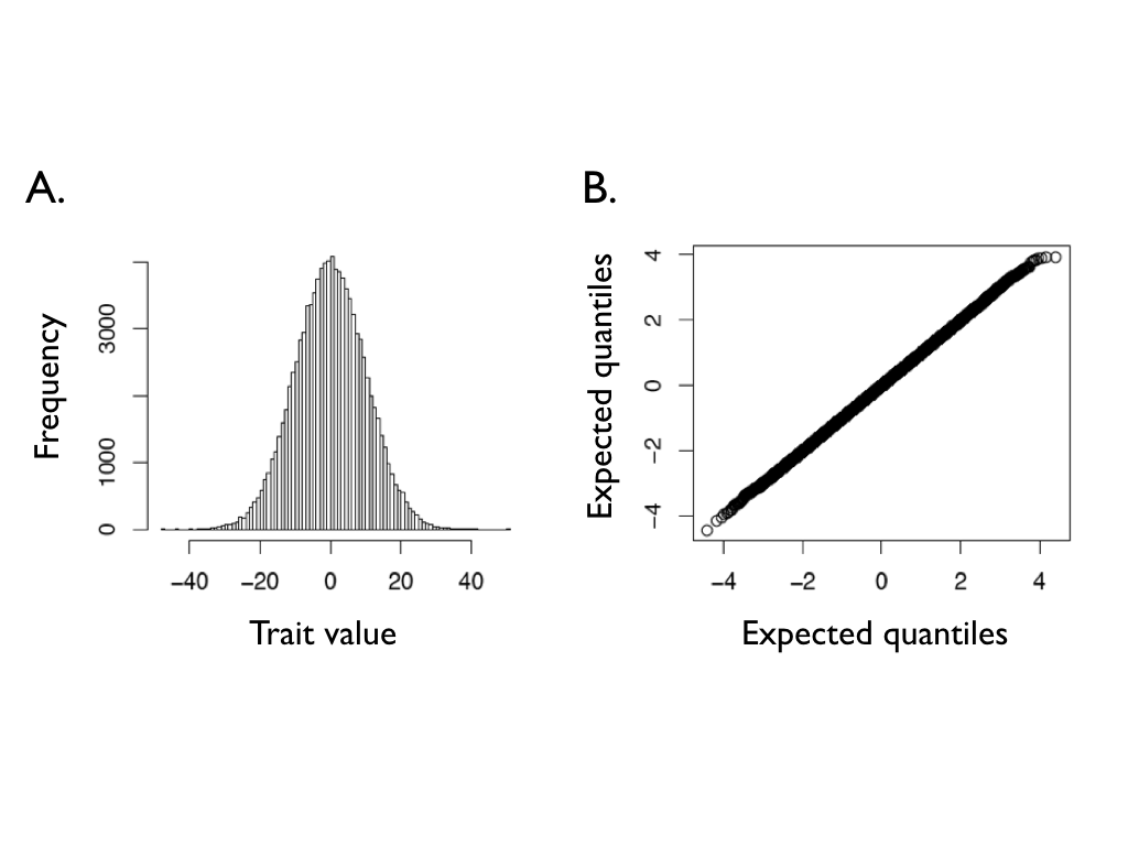
Figure 3.2. Ending character values from of 100,000 Brownian motion simulations with $\bar{z}(0) = 0$, t = 100, and σ2 = 1. Panel (A) shows a histogram of the outcome of these simulations, while panel (B) shows a normal Q-Q plot for these data. If the data follow a normal distribution, the points in the Q-Q plot should form a straight line. Image by the author, can be reused under a CC-BY-4.0 license.
Figure 3.3 shows how rate parameter σ2 affects the rate of spread of Brownian walks. The panels show sets of 100 Brownian motion simulations run over 1000 time units for σ2 = 1 (Panel A), σ2 = 5 (Panel B), and σ2 = 25 (Panel C). You can see that simulations with a higher rate parameter create a larger spread of trait values among simulations over the same amount of time.
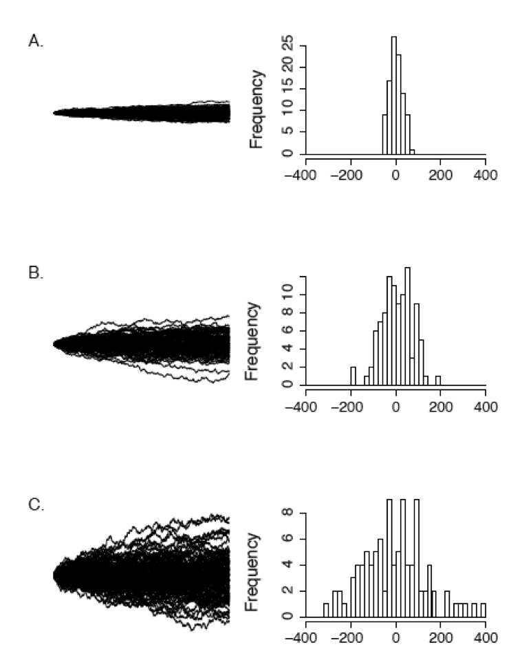
Figure 3.3. Examples of Brownian motion. Each plot shows 100 replicates of simulated Brownian motion with a common starting value and the same time interval t = 100. The rate parameter σ2 varies across the panels: (A) σ2 = 1 (B) σ2 = 10, and (C) σ2 = 25. The right-hand column shows a histogram of the distribution of ending values for each set of 100 simulations. Image by the author, can be reused under a CC-BY-4.0 license.
If we let $\bar{z}(t)$ be the value of our character at time t, then we can derive three main properties of Brownian motion. I will list all three, then explain each in turn.
- $E[\bar{z}(t)] = \bar{z}(0)$
- Each successive interval of the “walk” is independent
- $\bar{z}(t) \sim N(\bar{z}(0),\sigma^2 t)$
First, $E[\bar{z}(t)] = \bar{z}(0)$. This means that the expected value of the character at any time t is equal to the value of the character at time zero. Here the expected value refers to the mean of $\bar{z}(t)$ over many replicates. The intuitive meaning of this equation is that Brownian motion has no “trends,” and wanders equally in both positive and negative directions. If you take the mean of a large number of simulations of Brownian motion over any time interval, you will likely get a value close to $\bar{z}(0)$; as you increase the sample size, this mean will tend to get closer and closer to $\bar{z}(0)$.
Second, each successive interval of the “walk” is independent. Brownian motion is a process in continuous time, and so time does not have discrete “steps.” However, if you sample the process from time 0 to time t, and then again at time t + Δt, the change that occurs over these two intervals will be independent of one another. This is true of any two non-overlapping intervals sampled from a Brownian walk. It is worth noting that only the changes are independent, and that the value of the walk at time t + Δt – which we can write as $\bar{z}(t+\Delta t)$ - is not independent of the value of the walk at time t, $\bar{z}(t)$. But the differences between successive steps [e.g. $\bar{z}(t)-\bar{z}(0)$ and $\bar{z}(t+\Delta t) - \bar{z}(t)$] are independent of each other and of $\bar{z}(0)$.
Finally, $\bar{z}(t) \sim N(\bar{z}(0),\sigma^2 t)$.That is, the value of $\bar{z}(t)$ is drawn from a normal distribution with mean $\bar{z}(0)$ and variance σ2t. As we noted above, the parameter σ2 is important for Brownian motion models, as it describes the rate at which the process wanders through trait space. The overall variance of the process is that rate times the amount of time that has elapsed.
Section 3.3: Simple Quantitative Genetics Models for Brownian Motion
Section 3.3a: Brownian motion under genetic drift
The simplest way to obtain Brownian evolution of characters is when evolutionary change is neutral, with traits changing only due to genetic drift (e.g. Lande 1976). To show this, we will create a simple model. We will assume that a character is influenced by many genes, each of small effect, and that the value of the character does not affect fitness. Finally, we assume that mutations are random and have small effects on the character, as specified below. These assumptions probably seem unrealistic, especially if you are thinking of a trait like the body size of a lizard! But we will see later that we can also derive Brownian motion under other models, some of which involve selection.
Consider the mean value of this trait, $\bar{z}$, in a population with an effective population size of Ne (this is technically the variance effective population )2. Since there is no selection, the phenotypic character will change due only to mutations and genetic drift. We can model this process in a number of ways, but the simplest uses an "infinite alleles" model. Under this model, mutations occur randomly and have random phenotypic effects. We assume that mutations are drawn at random from a distribution with mean 0 and mutational variance σm2. This model assumes that the number of alleles is so large that there is effectively no chance of mutations happening to the same allele more than once - hence, "infinite alleles." The alleles in the population then change in frequency through time due to genetic drift. Drift and mutation together, then, determine the dynamics of the mean trait through time.
If we were to simulate this infinite alleles model many times, we would have a set of evolved populations. These populations would, on average, have the same mean trait value, but would differ from each other. Let’s try to derive how, exactly, these populations3 evolve.
If we consider a population evolving under this model, it is not difficult to show that the expected population phenotype after any amount of time is equal to the starting phenotype. This is because the phenotypes don’t matter for survival or reproduction, and mutations are assumed to be random and symmetrical. Thus,
(eq. 3.1)
$$
E[\bar{z}(t)] = \bar{z}(0)
$$
Note that this equation already matches the first property of Brownian motion.
Next, we need to also consider the variance of these mean phenotypes, which we will call the between-population phenotypic variance (σB2). Importantly, σB2 is the same quantity we earlier described as the “variance” of traits over time – that is, the variance of mean trait values across many independent “runs” of evolutionary change over a certain time period.
To calculate σB2, we need to consider variation within our model populations. Because of our simplifying assumptions, we can focus solely on additive genetic variance within each population at some time t, which we can denote as σa2. Additive genetic variance measures the total amount of genetic variation that acts additively (i.e. the contributions of each allele add together to predict the final phenotype). This excludes genetic variation involving interacions between alleles, such as dominance and epistasis (see Lynch and Walsh 1998 for a more detailed discussion). Additive genetic variance in a population will change over time due to genetic drift (which tends to decrease σa2) and mutational input (which tends to increase σa2). We can model the expected value of σa2 from one generation to the next as (Clayton and Robertson 1955; Lande 1979, 1980):
(eq. 3.2)
$$
E[\sigma_a^2 (t+1)]=(1-\frac{1}{2 N_e})E[\sigma_a^2 (t)]+\sigma_m^2
$$
where t is the elapsed time in generations, Ne is the effective population size, and σm2 is the mutational variance. There are two parts to this equation. The first, $(1-\frac{1}{2 N_e})E[\sigma_a^2 (t)]$, shows the decrease in additive genetic variance each generation due to genetic drift. The rate of decrease depends on effective population size, Ne, and the current level of additive variation. The second part of the equation describes how additive genetic variance increases due to new mutations (σm2) each generation.
If we assume that we know the starting value at time 0, σaStart2, we can calculate the expected additive genetic variance at any time t as:
(eq. 3.3)
$$
E[\sigma_a^2 (t)]={(1-\frac{1}{2 N_e})}^t [\sigma_{aStart}^2 - 2 N_e \sigma_m^2 ]+ 2 N_e \sigma_m^2
$$
Note that the first term in the above equation, ${(1-\frac{1}{2 N_e})}^t$, goes to zero as t becomes large. This means that additive genetic variation in the evolving populations will eventually reach an equilibrium between genetic drift and new mutations, so that additive genetic variation stops changing from one generation to the next. We can find this equilibrium by taking the limit of equation 3.3 as t becomes large.
(eq. 3.4)
limt → ∞E[σa2(t)] = 2Neσm2
Thus the equilibrium genetic variance depends on both population size and mutational input.
We can now derive the between-population phenotypic variance at time t, σB2(t). We will assume that σa2 is at equilibrium and thus constant (equation 3.4). Mean trait values in independently evolving populations will diverge from one another. Skipping some calculus, after some time period t has elapsed, the expected among-population variance will be (from Lande 1976):
(eq. 3.5)
$$
\sigma_B^2 (t)=\frac{t \sigma_a^2}{N_e}
$$
Substituting the equilibrium value of σa2 from equation 3.4 into equation 3.5 gives (Lande 1979, 1980):
(eq. 3.6)
$$
\sigma_B^2 (t)=\frac{t \sigma_a^2}{N_e} = \frac{t \cdot 2 N_e \sigma_m^2}{N_e} = 2 t \sigma_m^2
$$
Thie equation states that the variation among two diverging populations depends on twice the time since they have diverged and the rate of mutational input. Notice that for this model, the amount of variation among populations is independent of both the starting state of the populations and their effective population size. This model predicts, then, that long-term rates of evolution are dominated by the supply of new mutations to a population.
Even though we had to make particular specific assumptions for that derivation, Lynch and Hill (1986) show that equation 3.6 is a general result that holds under a range of models, even those that include dominance, linkage, nonrandom mating, and other processes. Equation 3.6 is somewhat useful, but we cannot often measure the mutational variance σm2 for any natural populations (but see Turelli 1984). By contrast, we sometimes do know the heritability of a particular trait. Heritability describes the proportion of total phenotypic variation within a population (σw2) that is due to additive genetic effects (σa2): $h^2=\frac{\sigma_a^2}{\sigma_w^2}$.
We can calculate the expected trait heritability for the infinite alleles model at mutational equilibrium. Substituting equation 3.4, we find that:
(eq. 3.7)
$$
h^2 = \frac{2 N_e \sigma_m^2}{\sigma_w^2}
$$
So that:
(eq. 3.8)
$$
\sigma_m^2 = \frac{h^2 \sigma_w^2}{2 N_e}
$$
Here, h2 is heritability, Ne the effective population size, and σw2 the within-population phenotypic variance, which differs from σa2 because it includes all sources of variation within populations, including both non-additive genetic effects and environmental effects. Substituting this expression for σw2 into equation 3.6, we have:
(eq. 3.9)
$$
\sigma_B^2 (t) = 2 \sigma_m^2 t = \frac{h^2 \sigma_w^2 t}{N_e}
$$
So, after some time interval t, the mean phenotype of a population has an expected value equal to the starting value, and a variance that depends positively on time, heritability, and trait variance, and negatively on effective population size.
To derive this result, we had to make particular assumptions about normality of new mutations that might seem quite unrealistic. It is worth noting that if phenotypes are affected by enough mutations, the central limit theorem guarantees that the distribution of phenotypes within populations will be normal – no matter what the underlying distribution of those mutations might be. We also had to assume that traits are neutral, a more dubious assumption that we relax below - where we will also show that there are other ways to get Brownian motion evolution than just genetic drift!
Note, finally, that this quantitative genetics model predicts that traits will evolve under a Brownian motion model. Thus, our quantitative genetics model has the same statistical properties of Brownian motion. We only need to translate one parameter: σ2 = h2σw2/Ne4.
Section 3.3b: Brownian motion under selection
We have shown that it is possible to relate a Brownian motion model directly to a quantitative genetics model of drift. In fact, there is some temptation to equate the two, and conclude that traits that evolve like Brownian motion are not under selection. However, this is incorrect. More specifically, an observation that a trait is evolving as expected under Brownian motion is not equivalent to saying that that trait is not under selection. This is because characters can also evolve as a Brownian walk even if there is strong selection – as long as selection acts in particular ways that maintain the properties of the Brownian motion model.
In general, the path followed by population mean trait values under mutation, selection, and drift depend on the particular way in which these processes occur. A variety of such models are considered by Hansen and Martins (1996). They identify three very different models that include selection where mean traits still evolve under an approximately Brownian model. Here I present univariate versions of the Hansen-Martins models, for simplicity; consult the original paper for multivariate versions. Note that all of these models require that the strength of selection is relatively weak, or else genetic variation of the character will be depleted by selection over time and the dynamics of trait evolution will change.
One model assumes that populations evolve due to directional selection, but the strength and direction of selection varies randomly from one generation to the next. We model selection each generation as being drawn from a normal distribution with mean 0 and variance σs2. Similar to our drift model, populations will again evolve under Brownian motion. However, in this case the Brownian motion parameters have a different interpretation:
(eq. 3.10)
$$
\sigma_B^2=(\frac{h^2 \sigma_W^2}{N_e} +\sigma_s^2)t
$$
In the particular case where variation in selection is much greater than variation due to drift, then:
(eq. 3.11)
σB2 ≈ σs2
That is, when selection is (on average) much stronger than drift, the rate of evolution is completely dominated by the selection term. This is not that far fetched, as many studies have shown selection in the wild that is both stronger than drift and commonly changing in both direction and magnitude from one generation to the next.
In a second model, Hansen and Martins (1996) consider a population subject to strong stabilizing selection for a particular optimal value, but where the position of the optimum itself changes randomly according to a Brownian motion process. In this case, population means can again be described by Brownian motion, but now the rate parameter reflects movement of the optimum rather than the action of mutation and drift. Specifically, if we describe movement of the optimum by a Brownian rate parameter σE2, then:
(eq. 3.12)
σB2 ≈ σE2
To obtain this result we must assume that there is at least a little bit of stabilizing selection (at least on the order of 1/tij where tij is the number of generations separating pairs of populations; Hansen and Martins 1996).
Again in this case, the population is under strong selection in any one generation, but long-term patterns of trait change can be described by Brownian motion. The rate of the random walk is totally determined by the action of selection rather than drift.
The important take-home point from both of these models is that the pattern of trait evolution through time under this model still follows a Brownian motion model, even though changes are dominated by selection and not drift. In other words, Brownian motion evolution does not imply that characters are not under selection!
Finally, Hansen and Martins (1996) consider the situation where populations evolve following a trend. In this case, we get evolution that is different from Brownian motion, but shares some key attributes. Consider a population under constant directional selection, s, so that:
(eq. 3.13)
$$
E[\bar{z}(t+1)]=\bar{z}(t) + h^2 s
$$
The variance among populations due to genetic drift after a single generation is then:
(eq. 3.14)
$$
\sigma_B^2 = \frac{h^2 \sigma_w^2}{N_e}
$$
Over some longer period of time, traits will evolve so that they have expected mean trait value that is normal with mean:
(eq. 3.15)
$$
E[\bar{z}(t)]=t \cdot (h^2 s)
$$
We can also calculate variance among species as:
(eq. 3.16)
$$
\sigma_B^2(t) = \frac{h^2 \sigma_w^2 t}{N_e}
$$
Note that the variance of this process is exactly identical to the variance among populations in a pure drift model (equation 3.9). Selection only changes the expectation for the species mean (of course, we assume that variation within populations and heritability are constant, which will only be true if selection is quite weak). Furthermore, with comparative methods, we are often considering a set of species and their traits in the present day, in which case they will all have experienced the same amount of evolutionary time (t) and have the same expected trait value. In fact, equations 3.14 and 3.16 are exactly the same as what we would expect under a pure-drift model in the same population, but starting with a trait value equal to $\bar{z}(0) = t \cdot (h^2 s)$ . That is, from the perspective of data only on living species, these two pure drift and linear selection models are statistically indistinguishable. The implications of this are striking: we can never find evidence for trends in evolution studying only living species (Slater et al. 2012).
In summary, we can describe three very different ways that traits might evolve under Brownian motion – pure drift, randomly varying selection, and varying stabilizing selection – and one model, constant directional selection, which creates patterns among extant species that are indistinguishable from Brownian motion. And there are more possible models out there that predict the same patterns. One can never tell these models apart by evaluating the qualitative pattern of evolution across species - they all predict the same pattern of Brownian motion evolution. The details differ, in that the models have Brownian motion rate parameters that differ from one another and relate to measurable quantities like population size and the strength of selection. Only by knowing something about these parameters can we distinguish among these possible scenarios.
You might notice that none of these “Brownian” models are particularly detailed, especially for modeling evolution over long time scales. You might even complain that these models are unrealistic. It is hard to imagine a case where a trait might be influenced only by random mutations of small effect over many alleles, or where selection would act in a truly random way from one generation to the next for millions of years. And you would be right! However, there are tremendous statistical benefits to using Brownian models for comparative analyses. Many of the results derived in this book, for example, are simple under Brownian motion but much more complex and different under other models. And it is also the case that some (but not all) methods are robust to modest violations of Brownian motion, in the same way that many standard statistical analyses are robust to minor variations of the assumptions of normality. In any case, we will proceed with models based on Brownian motion, keeping in mind these important caveats.
Section 3.4: Brownian motion on a phylogenetic tree
We can use the basic properties of Brownian motion model to figure out what will happen when characters evolve under this model on the branches of a phylogenetic tree. First, consider evolution along a single branch with length t1 (Figure 3.4A). In this case, we can model simple Brownian motion over time t1 and denote the starting value as $\bar{z}(0)$. If we evolve with some rate parameter σB2, then:
(eq. 3.17)
$$
E[\bar{z}(t)] \sim N(\bar{z}(0), \sigma_B^2 t_1)
$$
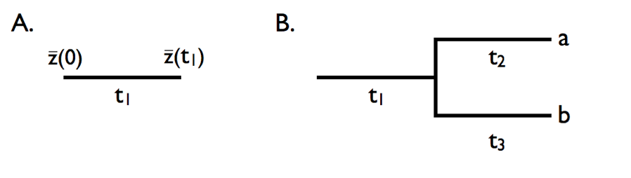
Figure 3.4. Brownian motion on a simple tree. A. Evolution in a single lineage over time period t1. B. Evolution on a phylogenetic tree relating species a and b, with branch lengths as given by t1, t2, and t3. Image by the author, can be reused under a CC-BY-4.0 license.
Now consider a small section of a phylogenetic tree including two species and an ancestral stem branch (Figure 3.4B). Assume a character evolves on that tree under Brownian motion, again with starting value $\bar{z}(0)$ and rate parameter σB2. First consider species a. The mean trait in that species $\bar{x}_a$ evolves under Brownian motion from the ancestor to species a over a total time of t1 + t2. Thus,
(eq. 3.18)
$$
\bar{x}_a \sim N[\bar{z}(0), \sigma_B^2 (t_1+t_2)]
$$
Similarly for species b, over a total time of t1 + t3
(eq. 3.19)
$$
\bar{x}_b \sim N[\bar{z}(0),\sigma_B^2 (t_1+t_3)]
$$
However, $\bar{x}_a$ and $\bar{x}_b$ are not independent of each other. Instead, the two species share one branch in common (branch 1). Each tip trait value can be thought of as an ancestral value plus the sum of two evolutionary changes: one (from branch 1) that is shared between the two species and one that is unique (branch 2 for species a and branch 3 for species b). In this case, mean trait values $\bar{x}_a$ and $\bar{x}_b$ will share similarity due to their shared evolutionary history. We can describe this similarity by calculating the covariance between the traits of species a and b. We note that:
(eq. 3.20)
$$
\begin{array}{lcr}
\bar{x}_a = \Delta \bar{x}_1 + \Delta \bar{x}_2\\
\bar{x}_b = \Delta \bar{x}_1 + \Delta \bar{x}_3\\
\end{array}
$$
Where $\Delta \bar{x}_1$, $\Delta \bar{x}_2$, and $\Delta \bar{x}_3$ represent evolution along the three branches in the tree, are all normally distributed with mean zero and variances σ2t1, σ2t2, and σ2t3, respectively. $\bar{x}_a$ and $\bar{x}_b$ are sums of normal random variables and are themselves normal. The covariance of these two terms is simply the variance of their shared term:
(eq. 3.21)
$$
cov(\bar{x}_a,\bar{x}_b)=var(\Delta \bar{x}_1)=\sigma_B^2 t_1
$$
It is also worth noting that we can describe the trait values for the two species as a single draw from a multivariate normal distribution. Each trait has the same expected value, $\bar{z}(0)$, and the two traits have a variance-covariance matrix:
(eq. 3.22)
$$
\begin{bmatrix}
\sigma^2 (t_1 + t_2) & \sigma^2 t_1 \\
\sigma^2 t_1 & \sigma^2 (t_1 + t_3) \\
\end{bmatrix}
= \sigma^2
\begin{bmatrix}
t_1 + t_2 & t_1 \\
t_1 & t_1 + t_3 \\
\end{bmatrix} = \sigma^2 \mathbf{C}
$$
The matrix C in equation 3.22 is commonly encountered in comparative biology, and will come up again in this book. We will call this matrix the phylogenetic variance-covariance matrix. This matrix has a special structure. For phylogenetic trees with n species, this is an n × n matrix, with each row and column corresponding to one of the n taxa in the tree. Along the diagonal are the total distances of each taxon from the root of the tree, while the off-diagonal elements are the total branch lengths shared by particular pairs of taxa. For example, C(1, 2) and C(2, 1) – which are equal because the matrix C is always symmetric – is the shared phylogenetic path length between the species in the first row – here, species a - and the species in the second row – here, species b. Under Brownian motion, these shared path lengths are proportional to the phylogenetic covariances of trait values. A full example of a phylogenetic variance-covariance matrix for a small tree is shown in Figure 3.5. This multivariate normal distribution completely describes the expected statistical distribution of traits on the tips of a phylogenetic tree if the traits evolve according to a Brownian motion model.
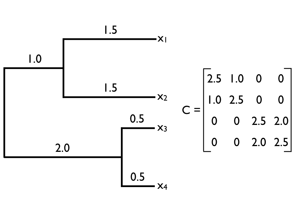
Figure 3.5. Example of a phylogenetic tree (left) and its associated phylogenetic variance-covariance matrix C (right). Image by the author, can be reused under a CC-BY-4.0 license.
Section 3.5: Multivariate Brownian motion
The Brownian motion model we described above was for a single character. However, we often want to consider more than one character at once. This requires the use of multivariate models. The situation is more complex than the univariate case – but not much! In this section I will derive the expectation for a set of (potentially correlated) traits evolving together under a multivariate Brownian motion model.
Character values across species can covary because of phylogenetic relationships, because different characters tend to evolve together, or both. Fortunately, we can generalize the model described above to deal with both of these types of covariation. To do this, we must combine two variance-covariance matrices. The first one, C, we have already seen; it describes the variances and covariances across species for single traits due to shared evolutionary history along the branches of a phylogentic tree. The second variance-covariance matrix, which we can call R, describes the variances and covariances across traits due to their tendencies to evolve together. For example, if a species of lizard gets larger due to the action of natural selection, then many of its other traits, like head and limb size, will get larger too due to allometry. The diagonal entries of the matrix R will provide our estimates of σi2, the net rate of evolution, for each trait, while off-diagonal elements, σij, represent evolutionary covariances between pairs of traits. We will denote number of species as n and the number of traits as m, so that C is n × n and R is m × m.
Our multivariate model of evolution has parameters that can be described by an m × 1 vector, a, containing the starting values for each trait – $\bar{z}_1(0)$, $\bar{z}_2(0)$, and so on, up to $\bar{z}_m(0)$, and an m × m matrix, R, described above. This model has m parameters for a and m ⋅ (m + 1)/2 parameters for R, for a total of m ⋅ (m + 3)/2 parameters.
Under our multivariate Brownian motion model, the joint distribution of all traits across all species still follows a multivariate normal distribution. We find the variance-covariance matrix that describes all characters across all species by combining the two matrices R and C into a single large matrix using the Kroeneker product:
(eq. 3.23)
V = R ⊗ C
This matrix V is n ⋅ m × n ⋅ m, and describes the variances and covariances of all traits across all species.
We can return to our example of evolution along a single branch (Figure 3.4a). Imagine that we have two characters that are evolving under a multivariate Brownian motion model. We state the parameters of the model as:
(eq. 3.24)
$$
\begin{array}{lcr}
\mathbf{a} =
\begin{bmatrix}
\bar{z}_1(0) \\
\bar{z}_2(0) \\
\end{bmatrix} \\
\mathbf{R} =
\begin{bmatrix}
\sigma_1^2 & \sigma_{12} \\
\sigma_{12} & \sigma_2^2 \\
\end{bmatrix} \\
\end{array}
$$
For a single branch, C = [t1], so:
(eq. 3.25)
$$
\mathbf{V} = \mathbf{R} \otimes \mathbf{C} =
\begin{bmatrix}
\sigma_1^2 & \sigma_{12} \\
\sigma_{12} & \sigma_2^2 \\
\end{bmatrix}
\otimes [t_1] =
\begin{bmatrix}
\sigma_1^2 t_1 & \sigma_{12} t_1 \\
\sigma_{12} t_1 & \sigma_2^2 t_1 \\
\end{bmatrix}
$$
The two traits follow a multivariate normal distribution with mean a and variance-covariance matrix V.
For the simple tree in figure 3.4b,
(eq. 3.26)
$$
\begin{array}{lcr}
\mathbf{V} = \mathbf{R} \otimes \mathbf{C} =
\begin{bmatrix}
\sigma_1^2 & \sigma_{12} \\
\sigma_{12} & \sigma_2^2 \\
\end{bmatrix}
\otimes
\begin{bmatrix}
t_1+t_2 & t_1 \\
t_1 & t_1+t_3 \\
\end{bmatrix} \\
=
\begin{bmatrix}
\sigma_1^2 (t_1+t_2) & \sigma_{12} (t_1+t_2) & \sigma_1^2 t_1 & \sigma_{12} t_1 \\
\sigma_{12} (t_1+t_2) & \sigma_2^2 (t_1+t_2) & \sigma_{12} t_1 & \sigma_2^2 t_1 \\
\sigma_1^2 t_1 & \sigma_{12} t_1 & \sigma_1^2 (t_1+t_3) & \sigma_{12} (t_1+t_3) \\
\sigma_{12} t_1 & \sigma_2^2 t_1 & \sigma_{12} (t_1+t_3) & \sigma_2^2 (t_1+t_3) \\
\end{bmatrix} \\
\end{array}
$$
Thus, the four trait values (two traits for two species) are drawn from a multivariate normal distribution with mean $a=[\bar{z}_1(0), \bar{z}_1(0), \bar{z}_2(0), \bar{z}_2(0)]$ and the variance-covariance matrix shown above.
Both univariate and multivariate Brownian motion models result in traits that follow multivariate normal distributions. This is statistically convenient, and in part explains the popularity of Brownian models in comparative biology.
Section 3.6: Simulating Brownian motion on trees
To simulate Brownian motion evolution on trees, we use the three properties of the model described above. For each branch on the tree, we can draw from a normal distribution (for a single trait) or a multivariate normal distribution (for more than one trait) to determine the evolution that occurs on that branch. We can then add these evolutionary changes together to obtain character states at every node and tip of the tree.
I will illustrate one such simulation for the simple tree depicted in figure 3.4b. We first set the ancestral character state to be $\bar{z}(0)$, which will then be the expected value for all the nodes and tips in the tree. This tree has three branches, so we draw three values from normal distributions. These normal distributions have mean zero and variances that are given by the rate of evolution and the branch length of the tree, as stated in equation 3.1. Note that we are modeling changes on these branches, so even if $\bar{z}(0) \neq 0$ the values for changes on branches are drawn from a distribution with a mean of zero. In the case of the tree in Figure 3.1, x1 ∼ N(0, σ2t1). Similarly, x2 ∼ N(0, σ2t2) and x3 ∼ N(0, σ2t3). If I set σ2 = 1 for the purposes of this example, I might obtain x1 = −1.6, x2 = 0.1, and x3 = −0.3. These values represent the evolutionary changes that occur along branches in the simulation. To calculate trait values for species, we add: xa = θ + x1 + x2 = 0 − 1.6 + 0.1 = −1.5, and xb = θ + x1 + x3 = 0 − 1.6 + −0.3 = −1.9.
This simulation algorithm works fine but is actually more complicated than it needs to be, especially for large trees. We already know that xa and xb come from a multivariate normal distribution with known mean vector and variance-covariance matrix. So, as a simple alternative, we can simply draw a vector from this distribution, and our tip values will have exactly the same statistical properties as if they were simulated on a phylogenetic tree. These two methods for simulating character evolution on trees are exactly equivalent to one another. In our small example, this alternative is not too much simpler than just adding the branches - but in some circumstances it is much easier to draw from a multivariate normal distribution.
Section 3.7: Summary
In this chapter, I introduced Brownian motion as a model of trait evolution. I first connected Brownian motion to a model of neutral genetic drift for traits that have no effect on fitness. However, as I demonstrated, Brownian motion can result from a variety of other models, some of which include natural selection. For example, traits will follow Brownian motion under selection is if the strength and direction of selection varies randomly through time. In other words, testing for a Brownian motion model with your data tells you nothing about whether or not the trait is under selection.
There is one general feature of all models that evolve in a Brownian way: they involve the action of a large number of very small “forces” pushing on characters. No matter the particular distribution of these small effects or even what causes them, if you add together enough of them you will obtain a normal distribution of outcomes and, sometimes, be able to model this process using Brownian motion. The main restriction might be the unbounded nature of Brownian motion – species are expected to become more and more different through time, without any limit, which must be unrealistic over very long time scales. We will deal with this issue in later chapters.
In summary, Brownian motion is mathematically tractable, and has convenient statistical properties. There are also some circumstances under which one would expect traits to evolve under a Brownian model. However, as we will see later in the book, one should view Brownian motion as an assumption that might not hold for real data sets.
Footnotes
1: More formally, the ball will move in two-dimensional Brownian motion, which describe movement both across and up and down the stadium rows. But if you consider just the movement in one direction - say, the distance of the ball from the field - then this is a simple single dimensional Brownian motion process as described here.
2: Variance effective population size is the effective population size of a model population with random mating, no substructure, and constant population size that would have quantitative genetic properties equal to our actual population. All of this is a bit beyond the scope of this book (but see Templeton 2006). But writing Ne instead of N allows us to develop the model without worrying about all of the extra assumptions we would have to make about how individuals mate and how populations are distributed over time and space.
3: In this book, we will typically consider variation among species rather than populations. However, we will also always assume that species are made up of one population, and so we can apply the same mathematical equations across species in a phylogenetic tree.
4: In some cases in the literature, the magnitude of trait change is expressed in within-population phenotypic standard deviations, $\sqrt{\sigma_w^2}$, per generation (Estes and Arnold 2007; e.g. Harmon et al. 2010). In that case, since dividing a random normal deviate by x is equivalent to dividing its variance by x2, we have σ2 = h2/Ne.
References
Clayton, G., and A. Robertson. 1955. Mutation and quantitative variation. Am. Nat. 89:151–158.
Estes, S., and S. J. Arnold. 2007. Resolving the paradox of stasis: Models with stabilizing selection explain evolutionary divergence on all timescales. Am. Nat. 169:227–244.
Hansen, T. F., and E. P. Martins. 1996. Translating between microevolutionary process and macroevolutionary patterns: The correlation structure of interspecific data. Evolution 50:1404–1417.
Harmon, L. J., J. B. Losos, T. Jonathan Davies, R. G. Gillespie, J. L. Gittleman, W. Bryan Jennings, K. H. Kozak, M. A. McPeek, F. Moreno-Roark, T. J. Near, and Others. 2010. Early bursts of body size and shape evolution are rare in comparative data. Evolution 64:2385–2396.
Hedges, B. S., and S. Kumar. 2009. The timetree of life. Oxford University Press, Oxford.
Lande, R. 1976. Natural selection and random genetic drift in phenotypic evolution. Evolution 30:314–334.
Lande, R. 1979. Quantitative genetic analysis of multivariate evolution, applied to brain:body size allometry. Evolution 33:402–416.
Lande, R. 1980. Sexual dimorphism, sexual selection, and adaptation in polygenic characters. Evolution 34:292–305.
Lynch, M., and W. G. Hill. 1986. Phenotypic evolution by neutral mutation. Evolution 40:915–935.
Lynch, M., and B. Walsh. 1998. Genetics and analysis of quantitative traits. Sinauer Sunderland, MA.
Slater, G. J., L. J. Harmon, and M. E. Alfaro. 2012. Integrating fossils with molecular phylogenies improves inference of trait evolution. Evolution 66:3931–3944. Blackwell Publishing Inc.
Templeton, A. R. 2006. Population genetics and microevolutionary theory. John Wiley & Sons.
Turelli, M. 1984. Heritable genetic variation via mutation-selection balance: Lerch’s zeta meets the abdominal bristle. Theor. Popul. Biol. 25:138–193.