Phylogenetic Comparative Methods learning from trees
Chapter 4: Fitting Brownian Motion Models to Single Characters
Section 4.1: Introduction
Mammals come in a wide variety of shapes and sizes. Some species are incredibly tiny. For example, the bumblebee bat, weighing in at 2 g, competes for the title of smallest mammal with the slightly lighter (but also slightly longer) Etruscan shrew (Hill 1974). Other species are huge, as anyone who has encountered a blue whale knows. Body size is important as a biological variable because it predicts so many other aspect of an animal’s life, from the physiology of heat exchange to the biomechanics of locomotion. Thus, the rate at which body size evolves is of great interest among mammalian biologists. Throughout this chapter, I will discuss the evolution of body size across different species of mammals. The data I will analyze is taken from Garland (1992).
Sometimes one might be interested in calculating the rate of evolution of a particular character like body size in a certain clade, say, mammals. You have a phylogenetic tree with branch lengths that are proportional to time, and data on the phenotypes of species on the tips of that tree. It is usually a good idea to log-transform your data if they involve a measurement from a living thing (see Box 4.1, below). If we assume that the character has been evolving under a Brownian motion model, we have two parameters to estimate: $\bar{z}(0)$, the starting value for the Brownian motion model – equivalent to the ancestral state of the character at the root of the tree – and σ2, the diffusion rate of the character. It is this latter parameter that is commonly considered as the rate of evolution for comparative approaches1.
Box 4.1: Biology under the log
One general rule for continuous traits in biology is to carry out a log-transformation (usually natural log, base e, denoted ln) of your data before undertaking any analysis. This also applies to comparative data. There are two main reasons for this, one statistical and the other biological. The statistical reason is that many methods assume that variables follow normal distributions. One can observe that, in general, measurements of species' traits have a distribution that is skewed to the right. A log-transformation will often result in trait distributions that are closer to normal. But why is this the case? The answer is related to the biological reason for log-transformation. When you log transform a variable, the new scale for that variable is a ratio scale, so that a certain differences between points reflects a constant ratio of the two numbers represented by the points. So, for example, if any two numbers are separated by 0.693 units on a natural log scale, one will be exactly two times the other. Ratio scales make sense for living things because it is usually percentage changes rather than absolute changes that matter. For example, a change in body size of 1 mm might matter a lot for a termite, but be irrelevant for an elephant; whereas a change in body size of 50% might be expected to matter for them both.
Section 4.2: Estimating rates using independent contrasts
The information required to estimate evolutionary rates is efficiently summarized in the early (but still useful) phylogenetic comparative method of independent contrasts (Felsenstein 1985). Independent contrasts summarize the amount of character change across each node in the tree, and can be used to estimate the rate of character change across a phylogeny. There is also a simple mathematical relationship between contrasts and maximum-likelihood rate estimates that I will discuss below.
We can understand the basic idea behind independent contrasts if we think about the branches in the phylogenetic tree as the historical “pathways” of evolution. Each branch on the tree represents a lineage that was alive at some time in the history of the Earth, and during that time experienced some amount of evolutionary change. We can imagine trying to measure that change initially by comparing sister taxa. We can compare the trait values of the two sister taxa by finding the difference in their trait values, and then compare that to the total amount of time they have had to evolve that difference. By doing this for all sister taxa in the tree, we will get an estimate of the average rate of character evolution ( 4.1A). But what about deeper nodes in the tree? We could use other non-sister species pairs, but then we would be counting some branches in the tree of life more than once (Figure 4.1B). Instead, we use a “pruning algorithm,” (Felsenstein 1985, Felsenstein (2004)) chopping off pairs of sister taxa to create a smaller tree (Figure 4.1C). Eventually, all of the nodes in the tree will be trimmed off – and the algorithm will finish. Independent contrasts provides a way to generalize the approach of comparing sister taxa so that we can quantify the rate of evolution throughout the whole tree.
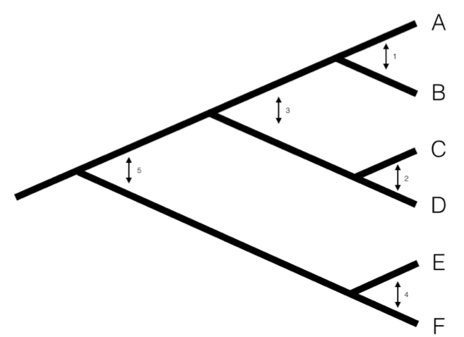
Figure 4.1. Pruning algorithm that can be used to identify five independent contrasts for a tree with six species (following Felsenstein 1985). The numbered order in this figure is only one of several possibilities that work; one can also prune the tree in the order 1, 2, 4, 3, 5 and get identical results. Image by the author, can be reused under a CC-BY-4.0 license.
A more precise algorithm describing how phylogenetic independent contrasts are calculated is provided in Box 4.2, below (from Felsenstein 1985). Each contrast can be described as an estimate of the direction and amount of evolutionary change across the nodes in the tree. PICs are calculated from the tips of the tree towards the root, as differences between trait values at the tips of the tree and/or calculated average values at internal nodes. The differences themselves are sometimes called “raw contrasts” (Felsenstein 1985). These raw contrasts will all be statistically independent of each other under a wide range of evolutionary models. In fact, as long as each lineage in a phylogenetic tree evolves independently of every other lineage, regardless of the evolutionary model, the raw contrasts will be independent of each other. However, people almost never use raw contrasts because they are not identically distributed; each raw contrast has a different expected distribution that depends on the model of evolution and the branch lengths of the tree. In particular, under Brownian motion we expect more change on longer branches of the tree. Felsenstein (1985) divided the raw contrasts by their expected standard deviation under a Brownian motion model, resulting in standardized contrasts. These standardized contrasts are, under a BM model, both independent and identically distributed, and can be used in a variety of statistical tests. Note that we must assume a Brownian motion model in order to standardize the contrasts; results derived from the contrasts, then, depend on this Brownian motion assumption.
Box 4.2: Algorithm for PICs
One can calculate PICs using the algorithm from Felsenstein (1985). I reproduce this algorithm below. Keep in mind that this is an iterative algorithm – you repeat the five steps below once for each contrast, or n − 1 times over the whole tree (see Figure 4.1C as an example).
Find two tips on the phylogeny that are adjacent (say nodes i and j) and have a common ancestor, say node k. Note that the choice of which node is i and which is j is arbitrary. As you will see, we will have to account for this “arbitrary direction” property of PICs in any analyses where we use them to do certian analyses!
- Compute the raw contrast, the difference between their two tip values: (eq. 4.1)
cij = xi − xj
- Under a Brownian motion model, cij has expectation zero and variance proportional to vi + vj.
- Calculate the standardized contrast by dividing the raw contrast by its variance (eq. 4.2)
$$ s_{ij} = \frac{c_{ij}}{v_i + v_j} = \frac{x_i - x_j}{v_i + v_j} $$
- Under a Brownian motion model, this contrast follows a normal distribution with mean zero and variance equal to the Brownian motion rate parameter σ2.
- Remove the two tips from the tree, leaving behind only the ancestor k, which now becomes a tip. Assign it the character value: (eq. 4.3)
$$ x_k = \frac{(1/v_i)x_i+(1/v_j)x_j}{1/v_1+1/v_j} $$
- It is worth noting that xk is a weighted average of xi and xj, but does not represent an ancestral state reconstruction, since the value is only influenced by species that descend directly from that node and not other relatives.
- Lengthen the branch below node k by increasing its length from vk to vk + vivj/(vi + vj). This accounts for the uncertainty in assigning a value to xk.
As mentioned above, we can apply the algorithm of independent contrasts to learn something about rates of body size evolution in mammals. We have a phylogenetic tree with branch lengths as well as body mass estimates for 49 species (Figure 4.2). If we ln-transform mass and then apply the method above to our data on mammal body size, we obtain a set of 48 standardized contrasts. A histogram of these contrasts is shown as Figure 4.2 (data from from Garland 1992).
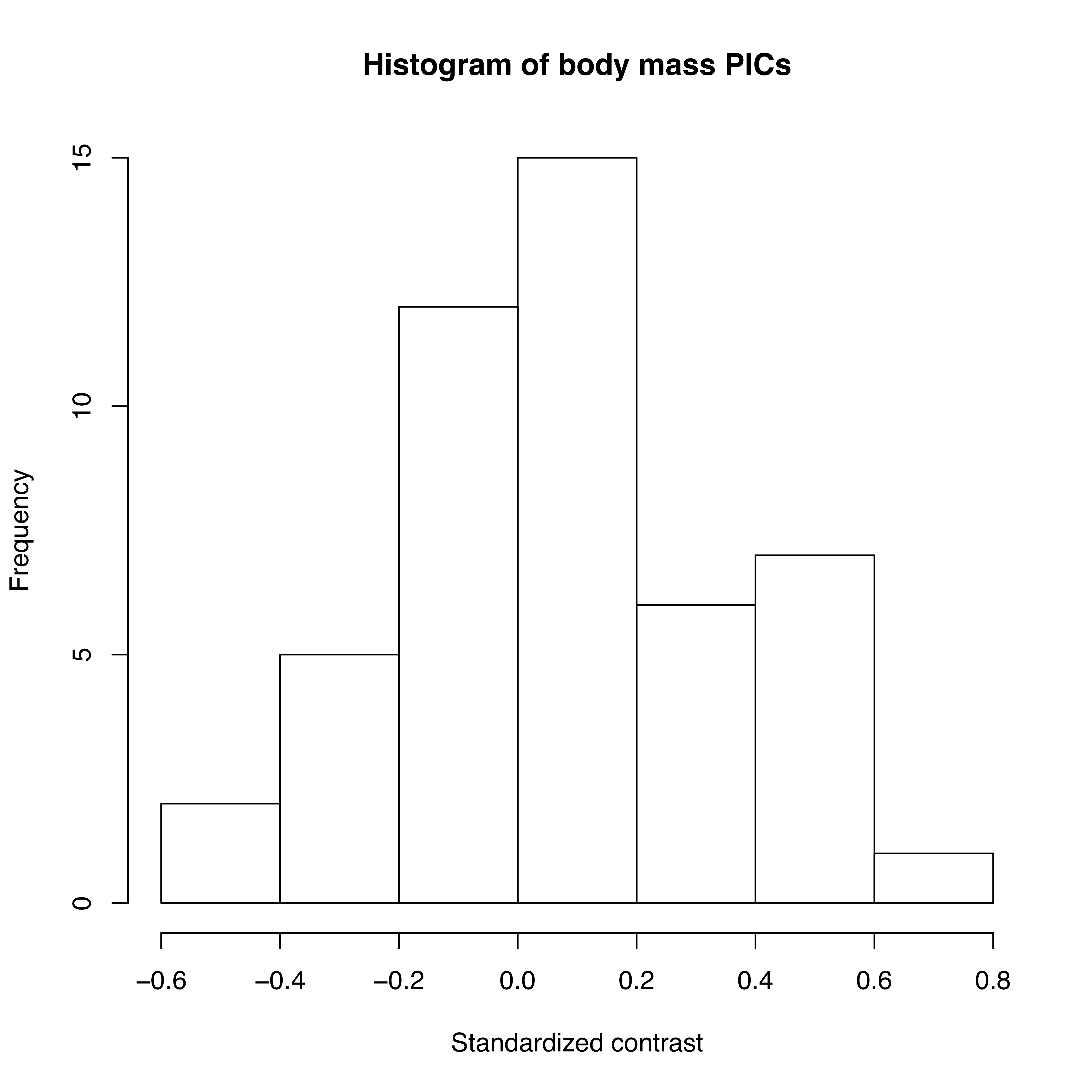
Figure 4.2. Histogram of PICs for ln-transformed mammal body mass on a phylogenetic tree with branch lengths in millions of years (data from Garland 1992). Image by the author, can be reused under a CC-BY-4.0 license.
Note that each contrast is an amount of change, xi − xj, divided by a branch length, vi + vj, which is a measure of time. Thus, PICs from a single trait can be used to estimate σ2, the rate of evolution under a Brownian model. The PIC estimate of the evolutionary rate is:
(eq. 4.4)
$$
\hat{\sigma}_{PIC}^2 = \frac{\sum{s_{ij}^2}}{n-1}
$$
That is, the PIC estimate of the evolutionary rate is the average of the n − 1 squared contrasts. This sum is taken over all sij, the standardized independent contrast across all (i, j) pairs of sister branches in the phylogenetic tree. For a fully bifurcating tree with n tips, there are exactly n − 1 such pairs. If you are statistically savvy, you might note that this formula looks a bit like a variance. In fact, if we state that the contrasts have a mean of 0 (which they must because Brownian motion has no overall trends), then this is a formula to estimate the variance of the contrasts.
If we calculate the mean sum of squared contrasts for the mammal body mass data, we obtain a rate estimate of $\hat{\sigma}_{PIC}^2$ = 0.09. We can put this into words: if we simulated mammalian body mass evolution under this model, we would expect the variance across replicated runs to increase by 0.09 per million years. Or, in more concrete terms, if we think about two lineages diverging from one another for a million years, we can draw changes in ln-body mass for both of them from a normal distribution with a variance of 0.09. Their difference, then, which is the amount of expected divergence, will be normal with a variance of 2 ⋅ 0.09 = 0.18. Thus, with 95% confidence, we can expect the two species to differ maximally by two standard deviations of this distribution, $2 \cdot \sqrt{0.18} = 0.85$. Since we are on a log scale, this amount of change corresponds to a factor of e2.68 = 2.3, meaning that one species will commonly be about twice as large (or small) as the other after just one million years.
Section 4.3: Estimating rates using maximum likelihood
We can also estimate the evolutionary rate by finding the maximum-likelihood parameter values for a Brownian motion model fit to our data. Recall that ML parameter values are those that maximize the likelihood of the data given our model (see Chapter 2).
We already know that under a Brownian motion model, tip character states are drawn from a multivariate normal distribution with a variance-covariance matrix, C, that is calculated based on the branch lengths and topology of the phylogenetic tree (see Chapter 3). We can calculate the likelihood of obtaining the data under our Brownian motion model using a standard formula for the likelihood of drawing from a multivariate normal distribution:
(eq. 4.5)
$$
L(\mathbf{x} | \bar{z}(0), \sigma^2, \mathbf{C}) =
\frac
{e^{-1/2 (\mathbf{x}-\bar{z}(0) \mathbf{1})^\intercal (\sigma^2 \mathbf{C})^{-1} (\mathbf{x}-\bar{z}(0) \mathbf{1})}}
{\sqrt{(2 \pi)^n det(\sigma^2 \mathbf{C})}}
$$
Here, our model parameters are σ2 and $\bar{z}(0)$, the root trait value. x is an n × 1 vector of trait values for the n tip species in the tree, with species in the same order as C, and 1 is an n × 1 column vector of ones. Note that (σ2C)−1 is the matrix inverse of the matrix σ2C
As an example, with the mammal data, we can calculate the likelihood for a model with parameter values σ2 = 1 and $\bar{z}(0) = 0$. We need to work with ln-likelihoods (lnL), both because the value here is so small and to facilitate future calculations, so: $lnL(\mathbf{x} | \bar{z}(0), \sigma^2, \mathbf{C}) = -116.2$.
To find the ML estimates of our model parameters, we need to find the parameter values that maximize that function. One (not very efficient) way to do this is to calculate the likelihood across a wide range of parameter values. One can then visualize the resulting likelihood surface and identify the maximum of the likelihood function. For example, the likelihood surface for the mammal body size data given a Brownian motion model is shown in Figure 4.3. Note that this surface has a peak around σ2 = 0.09 and $\bar{z}(0) = 4$. Inspecting the matrix of ML values, we find the highest ln-likelihood (-78.05) at σ2 = 0.089 and $\bar{z}(0) = 4.65$.
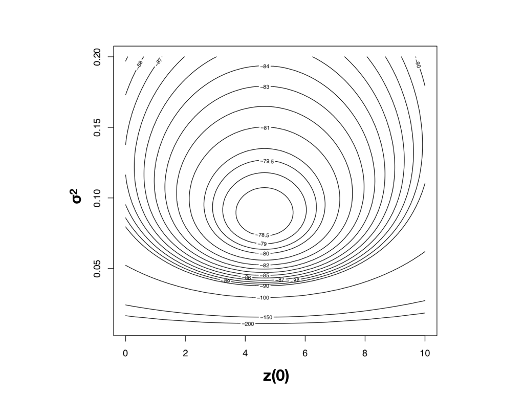
Figure 4.3. Likelihood surface for the evolution of mammalian body mass using the data from Garland (1992). Image by the author, can be reused under a CC-BY-4.0 license.
The calculation described above is inefficient, because we have to calculate likelihoods at a wide range of parameter values that are far from the optimum. A better strategy involves the use of optimization algorithms, a well-developed field of mathematical analysis (Nocedal and Wright 2006). These algorithms differ in their details, but we can illustrate how they work with a general example. Imagine that you are near Mt. St. Helens, and you are tasked with finding the peak of that mountain. It is foggy, but you can see the area around your feet and have an accurate altimeter. One strategy is to simply look at the slope of the mountain where you are standing, and climb uphill. If the slope is steep, you probably still are far from the top, and should climb fast; if the slope is shallow, you might be near the top of the mountain. It may seem obvious that this will get you to a local peak, but perhaps not the highest peak of Mt. St. Helens. Mathematical optimization schemes have this potential difficulty as well, but use some tricks to jump around in parameter space and try to find the overall highest peak as they climb. Details of actual optimization algorithms are beyond the scope of this book; for more information, see Nocedal and Wright (2006).
One simple example is based on Newton’s method of optimization [as implemented, for example, by the r function nlm()]. We can use this algorithm to quickly find accurate ML estimates2.
Using optimization algorithms we find a ML solution at $\hat{\sigma}_{ML}^2 = 0.08804487$ and $\hat{\bar{z}}(0) = 4.640571$, with lnL = −78.04942. Importantly, the solution can be found with only 10 likelihood calculations; this is the value of good optimization algorithms. I have plotted the path through parameter space taken by Newton’s method when searching for the optimum in Figure 4.4. Notice two things: first, that the function starts at some point and heads uphill on the likelihood surface until an optimum is found; and second, that this calculation requires many fewer steps (and much less time) than calculating the likelihood for a wide range of parameter values.
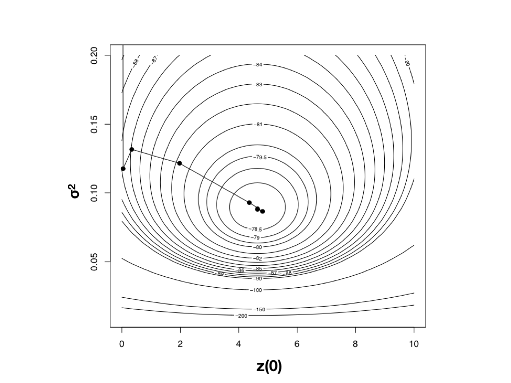
Figure 4.4. Likelihood surface for the evolution of mammalian body mass using the data from Garland (1992). Shown here is the path taken by the optimization algorithm to find the peak of the likelihood surface. The last five steps of this ten-step algorithm are too close together to be seen in this figure. Image by the author, can be reused under a CC-BY-4.0 license.
Using an optimization algorithm also has the added benefit of providing (approximate) confidence intervals for parameter values based on the Hessian of the likelihood surface. This approach assumes that the shape of the likelihood surface in the immediate vicinity of the peak can be approximated by a quadratic function, and uses the curvature of that function, as determined by the Hessian, to approximate the standard errors of parameter values (Burnham and Anderson 2003). If the surface is strongly peaked, the SEs will be small, while if the surface is very broad, the SEs will be large. For example, the likelihood surface around the ML values for mammal body size evolution has a Hessian of:
(eq. 4.6)
$$
H =
\begin{bmatrix}
-314.6 & -0.0026\\
-0.0026 & -0.99 \\
\end{bmatrix}
$$
This gives standard errors of 0.13 (for $\hat{\sigma}_{ML}^2$) and 0.72 [for $\hat{\bar{z}}(0)$]. If we assume the error around these estimates is approximately normal, we can create confidence estimates by adding and subtracting twice the standard error. We then obtain 95% CIs of 0.06 − 0.11 (for $\hat{\sigma}_{ML}^2$) and 3.22 − 6.06 [for $\hat{\bar{z}}(0)$].
The danger in optimization algorithms is that one can sometimes get stuck on local peaks. More elaborate algorithms repeated for multiple starting points can help solve this problem, but are not needed for simple Brownian motion on a tree as considered here. Numerical optimization is a difficult problem in phylogenetic comparative methods, especially for software developers.
In the particular case of fitting Brownian motion to trees, it turns out that even our fast algorithm for optimization was unnecessary. In this case, the maximum-likelihood estimate for each of these two parameters can be calculated analytically (O’Meara et al. 2006).
(eq. 4.7)
$$
\hat{\bar{z}}(0) = (\mathbf{1}^\intercal \mathbf{C}^{-1} \mathbf{1})^{-1} (\mathbf{1}^\intercal \mathbf{C}^{-1} \mathbf{x})
$$
and:
(eq. 4.8)
$$
\hat{\sigma}_{ML}^2 = \frac
{(\mathbf{x} - \hat{\bar{z}}(0) \mathbf{1})^\intercal \mathbf{C}^{-1} (\mathbf{x} - \hat{\bar{z}}(0) \mathbf{1})}
{n}
$$
where n is the number of taxa in the tree, C is the n × n variance-covariance matrix under Brownian motion for tip characters given the phylogenetic tree, x is an n × 1 vector of trait values for tip species in the tree, 1 is an n × 1 column vector of ones, $\hat{\bar{z}}(0)$ is the estimated root state for the character, and $\hat{\sigma}_{ML}^2$ is the estimated net rate of evolution.
Applying this approach to mammal body size, we obtain estimates that are exactly the same as our results from numeric optimization: $\hat{\sigma}_{ML}^2 = 0.088$ and $\hat{\bar{z}}(0) = 4.64$.
Equation (4.8) is biased, and will consistently estimate rates of evolution that are a little too small; an unbiased version based on restricted maximum likelihood (REML) and used by Garland (1992) and others is:
(eq. 4.9)$$ \hat{\sigma}_{REML}^2 = \frac {(\mathbf{x} - \hat{\bar{z}}(0) \mathbf{1})^\intercal \mathbf{C}^{-1} (\mathbf{x} - \hat{\bar{z}}(0) \mathbf{1})}{n-1} $$
This correction changes our estimate of the rate of body size in mammals from $\hat{\sigma}_{ML}^2 = 0.088$ to $\hat{\sigma}_{REML}^2 = 0.090$. Equation 4.8 is exactly identical to the estimated rate of evolution calculated using the average squared independent contrast, described above; that is, $\hat{\sigma}_{PIC}^2 = \hat{\sigma}_{REML}^2$. In fact, PICs are a formulation of a REML model. The “restricted” part of REML refers to the fact that these methods calculate likelihoods based on a transformed set of data where the effect of nuisance parameters has been removed. In this case, the nuisance parameter is the estimated root state $\hat{\bar{z}}(0)$ 3.
For the mammal body size example, we can further explore the difference between REML and ML in terms of statistical confidence intervals using likelihoods based on the contrasts. We assume, again, that the contrasts are all drawn from a normal distribution with mean 0 and unknown variance. If we again use Newton’s method for optimization, we find a maximum REML log-likelihood of -10.3 at $\hat{\sigma}_{REML}^2 = 0.090$. This returns a 1 × 1 matrix for the Hessian with a value of 2957.8, corresponding to a SE of 0.018. This slightly larger SE corresponds to 95% CI for $\hat{\sigma}_{REML}^2$ of 0.05 − 0.13.
In the context of comparative methods, REML has two main advantages. First, PICs treat the root state of the tree as a nuisance parameter. We typically have very little information about this root state, so that can be an advantage of the REML approach. Second, PICs are easy to calculate for very large phylogenetic trees because they do not require the construction (or inversion!) of any large variance-covariance matrices. This is important for big phylogenetic trees. Imagine that we had a phylogenetic tree of all vertebrates (~60,000 species) and wanted to calculate the rate of body size evolution. To use standard maximum likelihood, we have to calculate C, a matrix with 60, 000 × 60, 000 = 3.6 billion entries, and invert it to calculate C−1. To calculate PICs, by contrast, we only have to carry out on the order of 120,000 operations. Thankfully, there are now pruning algorithms to quickly calculate likelihoods for large trees under a variety of different models (see, e.g., FitzJohn 2012; Freckleton 2012; and Ho and Ané 2014).
Section 4.4: Bayesian approach to evolutionary rates
Finally, we can also use a Bayesian approach to fit Brownian motion models to data and to estimate the rate of evolution. This approach differs from the ML approach in that we will use explicit priors for parameter values, and then run an MCMC to estimate posterior distributions of parameter estimates. To do this, we will modify the basic algorithm for Bayesian MCMC (see Chapter 2) as follows:
Sample a set of starting parameter values, σ2 and $\bar{z}(0)$ from their prior distributions. For this example, we can set our prior distribution as uniform between 0 and 0.5 for σ2 and uniform from 0 to 10 for $\bar{z}(0)$.
- Given the current parameter values, select new proposed parameter values using the proposal density Q(p′|p). For both parameter values, we will use a uniform proposal density with width wp, so that: (eq. 4.10)
$$ Q(p'|p) \sim U(p-\frac{w_p}{2}, p+\frac{w_p}{2}) $$ - Calculate three ratios:
- The prior odds ratio, Rprior. This is the ratio of the probability of drawing the parameter values p and p’ from the prior. Since our priors are uniform, this is always 1.
- The proposal density ratio, Rproposal. This is the ratio of probability of proposals going from p to p’ and the reverse. We have already declared a symmetrical proposal density, so that Q(p′|p)=Q(p|p′) and Rproposal = 1.
- The likelihood ratio, Rlikelihood. This is the ratio of probabilities of the data given the two different parameter values. We can calculate these probabilities from equation 4.5 above. (eq. 4.11)
$$ R_{likelihood} = \frac{L(p'|D)}{L(p|D)} = \frac{P(D|p')}{P(D|p)} $$
Find the acceptance ratio, Raccept, which is product of the prior odds, proposal density ratio, and the likelihood ratio. In this case, both the prior odds and proposal density ratios are 1, so Raccept = Rlikelihood.
Draw a random number x from a uniform distribution between 0 and 1. If x < Raccept, accept the proposed value of both parameters; otherwise reject, and retain the current value of the two parameters.
Repeat steps 2-5 a large number of times.
Using the mammal body size data, I ran an MCMC with 10,000 generations, discarding the first 1000 as burn-in. Sampling every 10 generations, I obtain parameter estimates of $\hat{\sigma}_{bayes}^2 = 0.10$ (95% credible interval: 0.066 − 0.15) and $\hat{\bar{z}}(0) = 3.5$ (95% credible interval: 2.3 − 5.3; Figure 4.5).
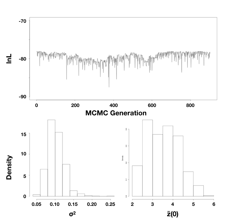
Figure 4.5. Bayesian analysis of body size evolution in mammals. Figure shows the likelihood profile (A) and posterior distributions for model parameters $\hat{\sigma}_{bayes}^2$ (B) and $\hat{\bar{z}}(0)$ (C). Image by the author, can be reused under a CC-BY-4.0 license.
Note that the parameter estimates from all three approaches (REML, ML, and Bayesian) were similar. Even the confidence/credible intervals varied a little bit but were of about the same size in all three cases. All of the approaches above are mathematically related and should, in general, return similar results. One might place higher value on the Bayesian credible intervals over confidence intervals from the Hessian of the likelihood surface, for two reasons: first, the Hessian leads to an estimate of the CI under certain conditions that may or may not be true for your analysis; and second, Bayesian credible intervals reflect overall uncertainty better than ML confidence intervals (see chapter 2).
Section 4.5: Summary
By fitting a Brownian motion model to phylogenetic comparative data, one can estimate the rate of evolution of a single character. In this chapter, I demonstrated three approaches to estimating that rate: PICs, maximum likelihood, and Bayesian MCMC. In the next chapter, we will discuss other models of evolution that can be fit to continuous characters on trees.
Footnotes
1: Throughout this chapter, when I say "rate" I will mean the Brownian motion parameter σ2. This is a little different from “traditional” estimates of evolutionary rate, like those estimated by paleontologists. For example, one might have measurements of trait in a series of fossils representing an evolutionary lineage sampled at different time periods. By calculating the amount of change over a given time interval, one can estimate an evolutionary rate. These rates can be expressed as Darwins (defined as the log-difference in trait values divided by time in years) or Haldanes (defined as the difference in trait values scaled by their standard deviations divided by time in generations). Both types of rates have been calculated from both fossil data and contemporary time-series data on evolution from both islands and lab experiments. Such rates best capture evolutionary trends, where the mean value of a trait is changing in a consistent way through time (for more information see review in Harmon 2014). Rates estimated by Brownian motion are a different type of “rate”, and some care must be taken to compare the two (see, e.g., Gingerich 1983).
2: Note that there are more complicated optimization algorithms that are useful for more difficult problems in comparative methods. In the case presented here, where the surface is smooth and has a single peak, almost any algorithm will work.
3:PICs are a transformation of the original data in which all information about the root state has been removed; our idea of what that root state might be has no effect on calculations using PICs. One can calculate the likelihood for the PIC REML method by assuming all of the standardized PICs are drawn from a normal distribution (eq. 4.5) with mean 0 and variance $\hat{\sigma}_{REML}^2$ (eq. 4.8). Alternatively, one can estimate the variance of the PICs directly, keeping in mind that one must use a mean of zero (eq. 4.4). These two methods give exactly the same results.
References
Burnham, K. P., and D. R. Anderson. 2003. Model selection and multimodel inference: A practical information theoretic approach. Springer Science & Business Media.
Felsenstein, J. 2004. Inferring phylogenies. Sinauer Associates, Inc., Sunderland, MA.
Felsenstein, J. 1985. Phylogenies and the comparative method. Am. Nat. 125:1–15.
FitzJohn, R. G. 2012. Diversitree: Comparative phylogenetic analyses of diversification in R. Methods Ecol. Evol. 3:1084–1092.
Freckleton, R. P. 2012. Fast likelihood calculations for comparative analyses. Methods Ecol. Evol. 3:940–947.
Garland, T., Jr. 1992. Rate tests for phenotypic evolution using phylogenetically independent contrasts. Am. Nat. 140:509–519.
Gingerich, P. D. 1983. Rates of evolution: Effects of time and temporal scaling. Science 222:159–161.
Harmon, L. J. 2014. Macroevolutionary rates. in The Princeton guide to evolution. Princeton University Press.
Hill, J. E. 1974. A new family, genus and species of bat (mammalia, chiroptera) from thailand. British Museum (Natural History).
Ho, L. S. T., and C. Ané. 2014. A linear-time algorithm for Gaussian and non-Gaussian trait evolution models. Syst. Biol. 63:397–408.
Nocedal, J., and S. Wright. 2006. Numerical optimization. Springer Science & Business Media.
O’Meara, B. C., C. Ané, M. J. Sanderson, and P. C. Wainwright. 2006. Testing for different rates of continuous trait evolution using likelihood. Evolution 60:922–933.