Phylogenetic Comparative Methods learning from trees
Chapter 2: Fitting Statistical Models to Data
Section 2.1: Introduction
Evolution is the product of a thousand stories. Individual organisms are born, reproduce, and die. The net result of these individual life stories over broad spans of time is evolution. At first glance, it might seem impossible to model this process over more than one or two generations. And yet scientific progress relies on creating simple models and confronting them with data. How can we evaluate models that consider evolution over millions of generations?
There is a solution: we can rely on the properties of large numbers to create simple models that represent, in broad brushstrokes, the types of changes that take place over evolutionary time. We can then compare these models to data in ways that will allow us to gain insights into evolution.
This book is about constructing and testing mathematical models of evolution. In my view the best comparative approaches have two features. First, the most useful methods emphasize parameter estimation over test statistics and P-values. Ideal methods fit models that we care about and estimate parameters that have a clear biological interpretation. To be useful, methods must also recognize and quantify uncertainty in our parameter estimates. Second, many useful methods involve model selection, the process of using data to objectively select the best model from a set of possibilities. When we use a model selection approach, we take advantage of the fact that patterns in empirical data sets will reject some models as implausible and support the predictions of others. This sort of approach can be a nice way to connect the results of a statistical analysis to a particular biological question.
In this chapter, I will first give a brief overview of standard hypothesis testing in the context of phylogenetic comparative methods. However, standard hypothesis testing can be limited in complex, real-world situations, such as those encountered commonly in comparative biology. I will then review two other statistical approaches, maximum likelihood and Bayesian analysis, that are often more useful for comparative methods. This latter discussion will cover both parameter estimation and model selection.
All of the basic statistical approaches presented here will be applied to evolutionary problems in later chapters. It can be hard to understand abstract statistical concepts without examples. So, throughout this part of the chapter, I will refer back to a simple example.
A common simple example in statistics involves flipping coins. To fit with the theme of this book, however, I will change this to flipping a lizard (needless to say, do not try this at home!). Suppose you have a lizard with two sides, “heads” and “tails.” You want to flip the lizard to help make decisions in your life. However, you do not know if this is a fair lizard, where the probability of obtaining heads is 0.5, or not. Perhaps, for example, lizards have a cat-like ability to right themselves when flipped. As an experiment, you flip the lizard 100 times, and obtain heads 63 of those times. Thus, 63 heads out of 100 lizard flips is your data; we will use model comparisons to try to see what these data tell us about models of lizard flipping.
Section 2.2: Standard statistical hypothesis testing
Standard hypothesis testing approaches focus almost entirely on rejecting null hypotheses. In the framework (usually referred to as the frequentist approach to statistics) one first defines a null hypothesis. This null hypothesis represents your expectation if some pattern, such as a difference among groups, is not present, or if some process of interest were not occurring. For example, perhaps you are interested in comparing the mean body size of two species of lizards, an anole and a gecko. Our null hypothesis would be that the two species do not differ in body size. The alternative, which one can conclude by rejecting that null hypothesis, is that one species is larger than the other. Another example might involve investigating two variables, like body size and leg length, across a set of lizard species1. Here the null hypothesis would be that there is no relationship between body size and leg length. The alternative hypothesis, which again represents the situation where the phenomenon of interest is actually occurring, is that there is a relationship with body size and leg length. For frequentist approaches, the alternative hypothesis is always the negation of the null hypothesis; as you will see below, other approaches allow one to compare the fit of a set of models without this restriction and choose the best amongst them.
The next step is to define a test statistic, some way of measuring the patterns in the data. In the two examples above, we would consider test statistics that measure the difference in mean body size among our two species of lizards, or the slope of the relationship between body size and leg length, respectively. One can then compare the value of this test statistic in the data to the expectation of this test statistic under the null hypothesis. The relationship between the test statistic and its expectation under the null hypothesis is captured by a P-value. The P-value is the probability of obtaining a test statistic at least as extreme as the actual test statistic in the case where the null hypothesis is true. You can think of the P-value as a measure of how probable it is that you would obtain your data in a universe where the null hypothesis is true. In other words, the P-value measures how probable it is under the null hypothesis that you would obtain a test statistic at least as extreme as what you see in the data. In particular, if the P-value is very large, say P = 0.94, then it is extremely likely that your data are compatible with this null hypothesis.
If the test statistic is very different from what one would expect under the null hypothesis, then the P-value will be small. This means that we are unlikely to obtain the test statistic seen in the data if the null hypothesis were true. In that case, we reject the null hypothesis as long as P is less than some value chosen in advance. This value is the significance threshold, α, and is almost always set to α = 0.05. By contrast, if that probability is large, then there is nothing “special” about your data, at least from the standpoint of your null hypothesis. The test statistic is within the range expected under the null hypothesis, and we fail to reject that null hypothesis. Note the careful language here – in a standard frequentist framework, you never accept the null hypothesis, you simply fail to reject it.
Getting back to our lizard-flipping example, we can use a frequentist approach. In this case, our particular example has a name; this is a binomial test, which assesses whether a given event with two outcomes has a certain probability of success. In this case, we are interested in testing the null hypothesis that our lizard is a fair flipper; that is, that the probability of heads pH = 0.5. The binomial test uses the number of “successes” (we will use the number of heads, H = 63) as a test statistic. We then ask whether this test statistic is either much larger or much smaller than we might expect under our null hypothesis. So, our null hypothesis is that pH = 0.5; our alternative, then, is that pH takes some other value: pH ≠ 0.5.
To carry out the test, we first need to consider how many "successes" we should expect if the null hypothesis were true. We consider the distribution of our test statistic (the number of heads) under our null hypothesis (pH = 0.5). This distribution is a binomial distribution (Figure 2.1).
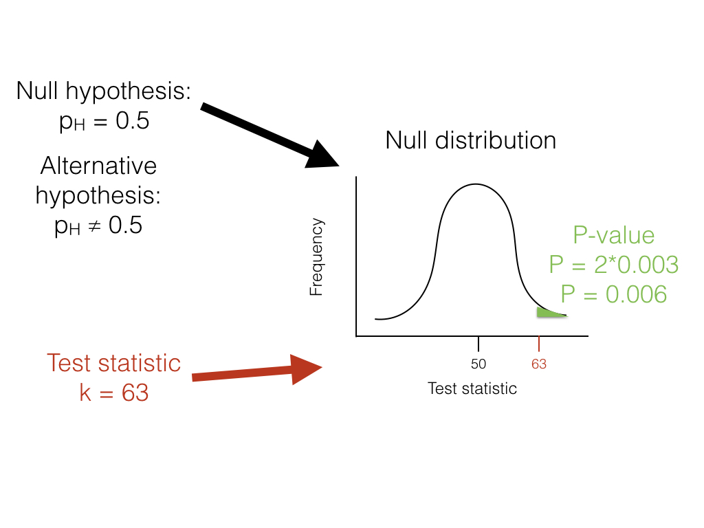
Figure 2.1. The unfair lizard. We use the null hypothesis to generate a null distribution for our test statistic, which in this case is a binomial distribution centered around 50. We then look at our test statistic and calculate the probability of obtaining a result at least as extreme as this value. Image by the author, can be reused under a CC-BY-4.0 license.
We can use the known probabilities of the binomial distribution to calculate our P-value. We want to know the probability of obtaining a result at least as extreme as our data when drawing from a binomial distribution with parameters p = 0.5 and n = 100. We calculate the area of this distribution that lies to the right of 63. This area, P = 0.003, can be obtained either from a table, from statistical software, or by using a relatively simple calculation. The value, 0.003, represents the probability of obtaining at least 63 heads out of 100 trials with pH = 0.5. This number is the P-value from our binomial test. Because we only calculated the area of our null distribution in one tail (in this case, the right, where values are greater than or equal to 63), then this is actually a one-tailed test, and we are only considering part of our null hypothesis where pH > 0.5. Such an approach might be suitable in some cases, but more typically we need to multiply this number by 2 to get a two-tailed test; thus, P = 0.006. This two-tailed P-value of 0.006 includes the possibility of results as extreme as our test statistic in either direction, either too many or too few heads. Since P < 0.05, our chosen α value, we reject the null hypothesis, and conclude that we have an unfair lizard.
In biology, null hypotheses play a critical role in many statistical analyses. So why not end this chapter now? One issue is that biological null hypotheses are almost always uninteresting. They often describe the situation where patterns in the data occur only by chance. However, if you are comparing living species to each other, there are almost always some differences between them. In fact, for biology, null hypotheses are quite often obviously false. For example, two different species living in different habitats are not identical, and if we measure them enough we will discover this fact. From this point of view, both outcomes of a standard hypothesis test are unenlightening. One either rejects a silly hypothesis that was probably known to be false from the start, or one “fails to reject” this null hypothesis2. There is much more information to be gained by estimating parameter values and carrying out model selection in a likelihood or Bayesian framework, as we will see below. Still, frequentist statistical approaches are common, have their place in our toolbox, and will come up in several sections of this book.
One key concept in standard hypothesis testing is the idea of statistical error. Statistical errors come in two flavors: type I and type II errors. Type I errors occur when the null hypothesis is true but the investigator mistakenly rejects it. Standard hypothesis testing controls type I errors using a parameter, α, which defines the accepted rate of type I errors. For example, if α = 0.05, one should expect to commit a type I error about 5% of the time. When multiple standard hypothesis tests are carried out, investigators often “correct” their P-values using Bonferroni correction. If you do this, then there is only a 5% chance of a single type I error across all of the tests being considered. This singular focus on type I errors, however, has a cost. One can also commit type II errors, when the null hypothesis is false but one fails to reject it. The rate of type II errors in statistical tests can be extremely high. While statisticians do take care to create approaches that have high power, traditional hypothesis testing usually fixes type I errors at 5% while type II error rates remain unknown. There are simple ways to calculate type II error rates (e.g. power analyses) but these are only rarely carried out. Furthermore, Bonferroni correction dramatically increases the type II error rate. This is important because – as stated by Perneger (1998) – “… type II errors are no less false than type I errors.” This extreme emphasis on controlling type I errors at the expense of type II errors is, to me, the main weakness of the frequentist approach3.
I will cover some examples of the frequentist approach in this book, mainly when discussing traditional methods like phylogenetic independent contrasts (PICs). Also, one of the model selection approaches used frequently in this book, likelihood ratio tests, rely on a standard frequentist set-up with null and alternative hypotheses.
However, there are two good reasons to look for better ways to do comparative statistics. First, as stated above, standard methods rely on testing null hypotheses that – for evolutionary questions - are usually very likely, a priori, to be false. For a relevant example, consider a study comparing the rate of speciation between two clades of carnivores. The null hypothesis is that the two clades have exactly equal rates of speciation – which is almost certainly false, although we might question how different the two rates might be. Second, in my opinion, standard frequentist methods place too much emphasis on P-values and not enough on the size of statistical effects. A small P-value could reflect either a large effect or very large sample sizes or both.
In summary, frequentist statistical methods are common in comparative statistics but can be limiting. I will discuss these methods often in this book, mainly due to their prevalent use in the field. At the same time, we will look for alternatives whenever possible.
Section 2.3: Maximum likelihood
Section 2.3a: What is a likelihood?
Since all of the approaches described in the remainer of this chapter involve calculating likelihoods, I will first briefly describe this concept. A good general review of likelihood is Edwards (1992). Likelihood is defined as the probability, given a model and a set of parameter values, of obtaining a particular set of data. That is, given a mathematical description of the world, what is the probability that we would see the actual data that we have collected?
To calculate a likelihood, we have to consider a particular model that may have generated the data. That model will almost always have parameter values that need to be specified. We can refer to this specified model (with particular parameter values) as a hypothesis, H. The likelihood is then:
(eq. 2.1)
L(H|D)=Pr(D|H)
Here, L and Pr stand for likelihood and probability, D for the data, and H for the hypothesis, which again includes both the model being considered and a set of parameter values. The | symbol stands for “given,” so equation 2.1 can be read as “the likelihood of the hypothesis given the data is equal to the probability of the data given the hypothesis.” In other words, the likelihood represents the probability under a given model and parameter values that we would obtain the data that we actually see.
For any given model, using different parameter values will generally change the likelihood. As you might guess, we favor parameter values that give us the highest probability of obtaining the data that we see. One way to estimate parameters from data, then, is by finding the parameter values that maximize the likelihood; that is, the parameter values that give the highest likelihood, and the highest probability of obtaining the data. These estimates are then referred to as maximum likelihood (ML) estimates. In an ML framework, we suppose that the hypothesis that has the best fit to the data is the one that has the highest probability of having generated that data.
For the example above, we need to calculate the likelihood as the probability of obtaining heads 63 out of 100 lizard flips, given some model of lizard flipping. In general, we can write the likelihood for any combination of H “successes” (flips that give heads) out of n trials. We will also have one parameter, pH, which will represent the probability of “success,” that is, the probability that any one flip comes up heads. We can calculate the likelihood of our data using the binomial theorem:
(eq. 2.2)
$$
L(H|D)=Pr(D|p)= {n \choose H} p_H^H (1-p_H)^{n-H}
$$
In the example given, n = 100 and H = 63, so:
(eq. 2.3)
$$
L(H|D)= {100 \choose 63} p_H^{63} (1-p_H)^{37}
$$

Figure 2.2. Likelihood surface for the parameter pH, given a coin that has been flipped as heads 63 times out of 100. Image by the author, can be reused under a CC-BY-4.0 license.
We can make a plot of the likelihood, L, as a function of pH (Figure 2.2). When we do this, we see that the maximum likelihood value of pH, which we can call $\hat{p}_H$, is at $\hat{p}_H = 0.63$. This is the “brute force” approach to finding the maximum likelihood: try many different values of the parameters and pick the one with the highest likelihood. We can do this much more efficiently using numerical methods as described in later chapters in this book.
We could also have obtained the maximum likelihood estimate for pH through differentiation. This problem is much easier if we work with the ln-likelihood rather than the likelihood itself (note that whatever value of pH that maximizes the likelihood will also maximize the ln-likelihood, because the log function is strictly increasing). So:
(eq. 2.4)
$$
\ln{L} = \ln{n \choose H} + H \ln{p_H}+ (n-H)\ln{(1-p_H)}
$$
Note that the natural log (ln) transformation changes our equation from a power function to a linear function that is easy to solve. We can differentiate:
(eq. 2.5)
$$
\frac{d \ln{L}}{dp_H} = \frac{H}{p_H} - \frac{(n-H)}{(1-p_H)}
$$
The maximum of the likelihood represents a peak, which we can find by setting the derivative $\frac{d \ln{L}}{dp_H}$ to zero. We then find the value of pH that solves that equation, which will be our estimate $\hat{p}_H$. So we have:
(eq. 2.6)
$$
\begin{array}{lcl}
\frac{H}{\hat{p}_H} - \frac{n-H}{1-\hat{p}_H} & = & 0\\
\frac{H}{\hat{p}_H} & = & \frac{n-H}{1-\hat{p}_H}\\
H (1-\hat{p}_H) & = & \hat{p}_H (n-H)\\
H-H\hat{p}_H & = & n\hat{p}_H-H\hat{p}_H\\
H & = & n\hat{p}_H\\
\hat{p}_H &=& H / n\\
\end{array}
$$
Notice that, for our simple example, H/n = 63/100 = 0.63, which is exactly equal to the maximum likelihood from figure 2.2.
Maximum likelihood estimates have many desirable statistical properties. It is worth noting, however, that they will not always return accurate parameter estimates, even when the data is generated under the actual model we are considering. In fact, ML parameters can sometimes be biased. To understand what this means, we need to formally introduce two new concepts: bias and precision. Imagine that we were to simulate datasets under some model A with parameter a. For each simulation, we then used ML to estimate the parameter $\hat{a}$ for the simulated data. The precision of our ML estimate tells us how different, on average, each of our estimated parameters $\hat{a}_i$ are from one another. Precise estimates are estimated with less uncertainty. Bias, on the other hand, measures how close our estimates $\hat{a}_i$ are to the true value a. If our ML parameter estimate is biased, then the average of the $\hat{a}_i$ will differ from the true value a. It is not uncommon for ML estimates to be biased in a way that depends on sample size, so that the estimates get closer to the truth as sample size increases, but can be quite far off in a particular direction when the number of data points is small compared to the number of parameters being estimated.
In our example of lizard flipping, we estimated a parameter value of $\hat{p}_H = 0.63$. For the particular case of estimating the parameter of a binomial distribution, our ML estimate is known to be unbiased. And this estimate is different from 0.5 – which was our expectation under the null hypothesis. So is this lizard fair? Or, alternatively, can we reject the null hypothesis that pH = 0.5? To evaluate this, we need to use model selection.
Section 2.3b: The likelihood ratio test
Model selection involves comparing a set of potential models and using some criterion to select the one that provides the “best” explanation of the data. Different approaches define “best” in different ways. I will first discuss the simplest, but also the most limited, of these techniques, the likelihood ratio test. Likelihood ratio tests can only be used in one particular situation: to compare two models where one of the models is a special case of the other. This means that model A is exactly equivalent to the more complex model B with parameters restricted to certain values. We can always identify the simpler model as the model with fewer parameters. For example, perhaps model B has parameters x, y, and z that can take on any values. Model A is the same as model B but with parameter z fixed at 0. That is, A is the special case of B when parameter z = 0. This is sometimes described as model A is nested within model B, since every possible version of model A is equal to a certain case of model B, but model B also includes more possibilities.
For likelihood ratio tests, the null hypothesis is always the simpler of the two models. We compare the data to what we would expect if the simpler (null) model were correct.
For example, consider again our example of flipping a lizard. One model is that the lizard is “fair:” that is, that the probability of heads is equal to 1/2. A different model might be that the probability of heads is some other value p, which could be 1/2, 1/3, or any other value between 0 and 1. Here, the latter (complex) model has one additional parameter, pH, compared to the former (simple) model; the simple model is a special case of the complex model when pH = 1/2.
For such nested models, one can calculate the likelihood ratio test statistic as
(eq. 2.7)
$$
\Delta = 2 \cdot \ln{\frac{L_1}{L_2}} = 2 \cdot (\ln{L_1}-\ln{L_2})
$$
Here, Δ is the likelihood ratio test statistic, L2 the likelihood of the more complex (parameter rich) model, and L1 the likelihood of the simpler model. Since the models are nested, the likelihood of the complex model will always be greater than or equal to the likelihood of the simple model. This is a direct consequence of the fact that the models are nested. If we find a particular likelihood for the simpler model, we can always find a likelihood equal to that for the complex model by setting the parameters so that the complex model is equivalent to the simple model. So the maximum likelihood for the complex model will either be that value, or some higher value that we can find through searching the parameter space. This means that the test statistic Δ will never be negative. In fact, if you ever obtain a negative likelihood ratio test statistic, something has gone wrong – either your calculations are wrong, or you have not actually found ML solutions, or the models are not actually nested.
To carry out a statistical test comparing the two models, we compare the test statistic Δ to its expectation under the null hypothesis. When sample sizes are large, the null distribution of the likelihood ratio test statistic follows a chi-squared (χ2) distribution with degrees of freedom equal to the difference in the number of parameters between the two models. This means that if the simpler hypothesis were true, and one carried out this test many times on large independent datasets, the test statistic would approximately follow this χ2 distribution. To reject the simpler (null) model, then, one compares the test statistic with a critical value derived from the appropriate χ2 distribution. If the test statistic is larger than the critical value, one rejects the null hypothesis. Otherwise, we fail to reject the null hypothesis. In this case, we only need to consider one tail of the χ2 test, as every deviation from the null model will push us towards higher Δ values and towards the right tail of the distribution.
For the lizard flip example above, we can calculate the ln-likelihood under a hypothesis of pH = 0.5 as:
(eq. 2.8)
$$
\begin{array}{lcl}
\ln{L_1} &=& \ln{\left(\frac{100}{63}\right)} + 63 \cdot \ln{0.5} + (100-63) \cdot \ln{(1-0.5)} \nonumber \\
\ln{L_1} &=& -5.92\nonumber\\
\end{array}
$$
We can compare this to the likelihood of our maximum-likelihood estimate :
(eq. 2.9)
$$
\begin{array}{lcl}
\ln{L_2} &=& \ln{\left(\frac{100}{63}\right)} + 63 \cdot \ln{0.63} + (100-63) \cdot \ln{(1-0.63)} \nonumber \\
\ln{L_2} &=& -2.50\nonumber
\end{array}
$$
We then calculate the likelihood ratio test statistic:
(eq. 2.10)
$$
\begin{array}{lcl}
\Delta &=& 2 \cdot (\ln{L_2}-\ln{L_1}) \nonumber \\
\Delta &=& 2 \cdot (-2.50 - -5.92) \nonumber \\
\Delta &=& 6.84\nonumber
\end{array}
$$
If we compare this to a χ2 distribution with one d.f., we find that P = 0.009. Because this P-value is less than the threshold of 0.05, we reject the null hypothesis, and support the alternative. We conclude that this is not a fair lizard. As you might expect, this result is consistent with our answer from the binomial test in the previous section. However, the approaches are mathematically different, so the two P-values are not identical.
Although described above in terms of two competing hypotheses, likelihood ratio tests can be applied to more complex situations with more than two competing models. For example, if all of the models form a sequence of increasing complexity, with each model a special case of the next more complex model, one can compare each pair of hypotheses in sequence, stopping the first time the test statistic is non-significant. Alternatively, in some cases, hypotheses can be placed in a bifurcating choice tree, and one can proceed from simple to complex models down a particular path of paired comparisons of nested models. This approach is commonly used to select models of DNA sequence evolution (Posada and Crandall 1998).
Section 2.3c: The Akaike information criterion (AIC)
You might have noticed that the likelihood ratio test described above has some limitations. Especially for models involving more than one parameter, approaches based on likelihood ratio tests can only do so much. For example, one can compare a series of models, some of which are nested within others, using an ordered series of likelihood ratio tests. However, results will often depend strongly on the order in which tests are carried out. Furthermore, often we want to compare models that are not nested, as required by likelihood ratio tests. For these reasons, another approach, based on the Akaike Information Criterion (AIC), can be useful.
The AIC value for a particular model is a simple function of the likelihood L and the number of parameters k:
(eq. 2.11)
AIC = 2k − 2lnL
This function balances the likelihood of the model and the number of parameters estimated in the process of fitting the model to the data. One can think of the AIC criterion as identifying the model that provides the most efficient way to describe patterns in the data with few parameters. However, this shorthand description of AIC does not capture the actual mathematical and philosophical justification for equation (2.11). In fact, this equation is not arbitrary; instead, its exact trade-off between parameter numbers and log-likelihood difference comes from information theory (for more information, see Burnham and Anderson 2003, Akaike (1998)).
The AIC equation (2.11) above is only valid for quite large sample sizes relative to the number of parameters being estimated (for n samples and k parameters, n/k > 40). Most empirical data sets include fewer than 40 independent data points per parameter, so a small sample size correction should be employed:
(eq. 2.12)
$$
AIC_C = AIC + \frac{2k(k+1)}{n-k-1}
$$
This correction penalizes models that have small sample sizes relative to the number of parameters; that is, models where there are nearly as many parameters as data points. As noted by Burnham and Anderson (2003), this correction has little effect if sample sizes are large, and so provides a robust way to correct for possible bias in data sets of any size. I recommend always using the small sample size correction when calculating AIC values.
To select among models, one can then compare their AICc scores, and choose the model with the smallest value. It is easier to make comparisons in AICc scores between models by calculating the difference, ΔAICc. For example, if you are comparing a set of models, you can calculate ΔAICc for model i as:
(eq. 2.13)
ΔAICci = AICci − AICcmin
where AICci is the AICc score for model i and AICcmin is the minimum AICc score across all of the models.
As a broad rule of thumb for comparing AIC values, any model with a ΔAICci of less than four is roughly equivalent to the model with the lowest AICc value. Models with ΔAICci between 4 and 8 have little support in the data, while any model with a ΔAICci greater than 10 can safely be ignored.
Additionally, one can calculate the relative support for each model using Akaike weights. The weight for model i compared to a set of competing models is calculated as:
(eq. 2.14)
$$
w_i = \frac{e^{-\Delta AIC_{c_i}/2}}{\sum_i{e^{-\Delta AIC_{c_i}/2}}}
$$
The weights for all models under consideration sum to 1, so the wi for each model can be viewed as an estimate of the level of support for that model in the data compared to the other models being considered.
Returning to our example of lizard flipping, we can calculate AICc scores for our two models as follows:
(eq. 2.15)
$$
\begin{array}{lcl}
AIC_1 &=& 2 k_1 - 2 ln{L_1} = 2 \cdot 0 - 2 \cdot -5.92 \\\
AIC_1 &=& 11.8 \\\
AIC_2 &=& 2 k_2 - 2 ln{L_2} = 2 \cdot 1 - 2 \cdot -2.50 \\\
AIC_2 &=& 7.0 \\\
\end{array}
$$
Our example is a bit unusual in that model one has no estimated parameters; this happens sometimes but is not typical for biological applications. We can correct these values for our sample size, which in this case is n = 100 lizard flips:
(eq. 2.16)
$$
\begin{array}{lcl}
AIC_{c_1} &=& AIC_1 + \frac{2 k_1 (k_1 + 1)}{n - k_1 - 1} \\\
AIC_{c_1} &=& 11.8 + \frac{2 \cdot 0 (0 + 1)}{100-0-1} \\\
AIC_{c_1} &=& 11.8 \\\
AIC_{c_2} &=& AIC_2 + \frac{2 k_2 (k_2 + 1)}{n - k_2 - 1} \\\
AIC_{c_2} &=& 7.0 + \frac{2 \cdot 1 (1 + 1)}{100-1-1} \\\
AIC_{c_2} &=& 7.0 \\\
\end{array}
$$
Notice that, in this particular case, the correction did not affect our AIC values, at least to one decimal place. This is because the sample size is large relative to the number of parameters. Note that model 2 has the smallest AICc score and is thus the model that is best supported by the data. Noting this, we can now convert these AICc scores to a relative scale:
(eq. 2.17)
$$
\begin{array}{lcl}
\Delta AIC_{c_1} &=& AIC_{c_1}-AIC{c_{min}} \\\
&=& 11.8-7.0 \\\
&=& 4.8 \\\
\end{array}
$$
$$
\begin{array}{lcl}
\Delta AIC_{c_2} &=& AIC_{c_2}-AIC{c_{min}} \\\
&=& 7.0-7.0 \\\
&=& 0 \\\
\end{array}
$$
Note that the ΔAICci for model 1 is greater than four, suggesting that this model (the “fair” lizard) has little support in the data. This is again consistent with all of the results that we've obtained so far using both the binomial test and the likelihood ratio test. Finally, we can use the relative AICc scores to calculate Akaike weights:
(eq. 2.18)
$$
\begin{array}{lcl}
\sum_i{e^{-\Delta_i/2}} &=& e^{-\Delta_1/2} + e^{-\Delta_2/2} \\\
&=& e^{-4.8/2} + e^{-0/2} \\\
&=& 0.09 + 1 \\\
&=& 1.09 \\\
\end{array}
$$
$$
\begin{array}{lcl}
w_1 &=& \frac{e^{-\Delta AIC_{c_1}/2}}{\sum_i{e^{-\Delta AIC_{c_i}/2}}} \\\
&=& \frac{0.09}{1.09} \\\
&=& 0.08
\end{array}
$$
$$
\begin{array}{lcl}
w_2 &=& \frac{e^{-\Delta AIC_{c_2}/2}}{\sum_i{e^{-\Delta AIC_{c_i}/2}}} \\\
&=& \frac{1.00}{1.09} \\\
&=& 0.92
\end{array}
$$
Our results are again consistent with the results of the likelihood ratio test. The relative likelihood of an unfair lizard is 0.92, and we can be quite confident that our lizard is not a fair flipper.
AIC weights are also useful for another purpose: we can use them to get model-averaged parameter estimates. These are parameter estimates that are combined across different models proportional to the support for those models. As a thought example, imagine that we are considering two models, A and B, for a particular dataset. Both model A and model B have the same parameter p, and this is the parameter we are particularly interested in. In other words, we do not know which model is the best model for our data, but what we really need is a good estimate of p. We can do that using model averaging. If model A has a high AIC weight, then the model-averaged parameter estimate for p will be very close to our estimate of p under model A; however, if both models have about equal support then the parameter estimate will be close to the average of the two different estimates. Model averaging can be very useful in cases where there is a lot of uncertainty in model choice for models that share parameters of interest. Sometimes the models themselves are not of interest, but need to be considered as possibilities; in this case, model averaging lets us estimate parameters in a way that is not as strongly dependent on our choice of models.
Section 2.4: Bayesian statistics
Section 2.4a: Bayes Theorem
Recent years have seen tremendous growth of Bayesian approaches in reconstructing phylogenetic trees and estimating their branch lengths. Although there are currently only a few Bayesian comparative methods, their number will certainly grow as comparative biologists try to solve more complex problems. In a Bayesian framework, the quantity of interest is the posterior probability, calculated using Bayes' theorem:
(eq. 2.19)
$$
Pr(H|D) = \frac{Pr(D|H) \cdot Pr(H)}{Pr(D)}
$$
The benefit of Bayesian approaches is that they allow us to estimate the probability that the hypothesis is true given the observed data, Pr(H|D). This is really the sort of probability that most people have in mind when they are thinking about the goals of their study. However, Bayes theorem also reveals a cost of this approach. Along with the likelihood, Pr(D|H), one must also incorporate prior knowledge about the probability that any given hypothesis is true - Pr(H). This represents the prior belief that a hypothesis is true, even before consideration of the data at hand. This prior probability must be explicitly quantified in all Bayesian statistical analyses. In practice, scientists often seek to use “uninformative” priors that have little influence on the posterior distribution - although even the term "uninformative" can be confusing, because the prior is an integral part of a Bayesian analysis. The term Pr(D) is also an important part of Bayes theorem, and can be calculated as the probability of obtaining the data integrated over the prior distributions of the parameters:
(eq. 2.20)
Pr(D)=∫HPr(H|D)Pr(H)dH
However, Pr(D) is constant when comparing the fit of different models for a given data set and thus has no influence on Bayesian model selection under most circumstances (and all the examples in this book).
In our example of lizard flipping, we can do an analysis in a Bayesian framework. For model 1, there are no free parameters. Because of this, Pr(H)=1 and Pr(D|H)=P(D), so that Pr(H|D)=1. This may seem strange but what the result means is that our data has no influence on the structure of the model. We do not learn anything about a model with no free parameters by collecting data!
If we consider model 2 above, the parameter pH must be estimated. We can set a uniform prior between 0 and 1 for pH, so that f(pH)=1 for all pH in the interval [0,1]. We can also write this as “our prior for ph is U(0,1)”. Then:
(eq. 2.21)
$$
Pr(H|D) = \frac{Pr(D|H) \cdot Pr(H)}{Pr(D)} = \frac{P(H|p_H,N) f(p_H)}{\int_{0}^{1} P(H|p_H,N) f(p_h) dp_H}
$$
Next we note that Pr(D|H) is the likelihood of our data given the model, which is already stated above as equation 2.2. Plugging this into our equation, we have:
(eq. 2.22)
$$
Pr(H|D) = \frac{\binom{N}{H} p_H^H (1-p_H)^{N-H}}{\int_{0}^{1} \binom{N}{H} p_H^H (1-p_H)^{N-H} dp_H}
$$
This ugly equation actually simplifies to a beta distribution, which can be expressed more simply as:
(eq. 2.23)
$$
Pr(H|D) = \frac{(N+1)!}{H!(N-H)!} p_H^H (1-p_H)^{N-H}
$$
We can compare this posterior distribution of our parameter estimate, pH, given the data, to our uniform prior (Figure 2.3). If you inspect this plot, you see that the posterior distribution is very different from the prior – that is, the data have changed our view of the values that parameters should take. Again, this result is qualitatively consistent with both the frequentist and ML approaches described above. In this case, we can see from the posterior distribution that we can be quite confident that our parameter pH is not 0.5.
As you can see from this example, Bayes theorem lets us combine our prior belief about parameter values with the information from the data in order to obtain a posterior. These posterior distributions are very easy to interpret, as they express the probability of the model parameters given our data. However, that clarity comes at a cost of requiring an explicit prior. Later in the book we will learn how to use this feature of Bayesian statistics to our advantage when we actually do have some prior knowledge about parameter values.
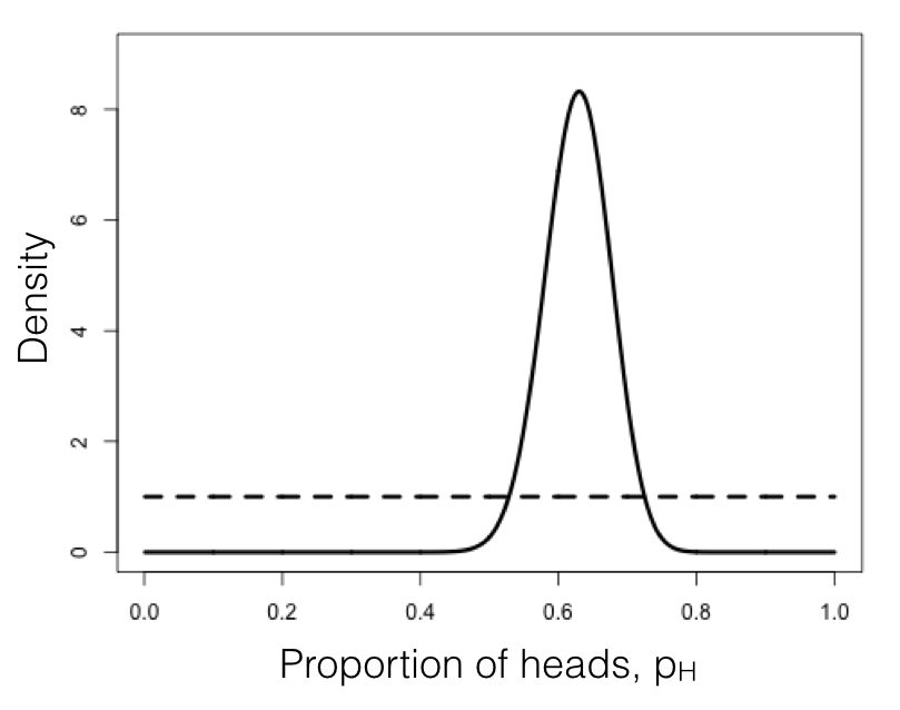
Figure 2.3. Bayesian prior (dotted line) and posterior (solid line) distributions for lizard flipping. Image by the author, can be reused under a CC-BY-4.0 license.
Section 2.4b: Bayesian MCMC
The other main tool in the toolbox of Bayesian comparative methods is the use of Markov-chain Monte Carlo (MCMC) tools to calculate posterior probabilities. MCMC techniques use an algorithm that uses a “chain” of calculations to sample the posterior distribution. MCMC requires calculation of likelihoods but not complicated mathematics (e.g. integration of probability distributions, as in equation 2.22), and so represents a more flexible approach to Bayesian computation. Frequently, the integrals in equation 2.21 are intractable, so that the most efficient way to fit Bayesian models is by using MCMC. Also, setting up an MCMC is, in my experience, easier than people expect!
An MCMC analysis requires that one constructs and samples from a Markov chain. A Markov chain is a random process that changes from one state to another with certain probabilities that depend only on the current state of the system, and not what has come before. A simple example of a Markov chain is the movement of a playing piece in the game Chutes and Ladders; the position of the piece moves from one square to another following probabilities given by the dice and the layout of the game board. The movement of the piece from any square on the board does not depend on how the piece got to that square.
Some Markov chains have an equilibrium distribution, which is a stable probability distribution of the model’s states after the chain has run for a very long time. For Bayesian analysis, we use a technique called a Metropolis-Hasting algorithm to construct a special Markov chain that has an equilibrium distribution that is the same as the Bayesian posterior distribution of our statistical model. Then, using a random simulation on this chain (this is the Markov-chain Monte Carlo, MCMC), we can sample from the posterior distribution of our model.
In simpler terms: we use a set of well-defined rules. These rules let us walk around parameter space, at each step deciding whether to accept or reject the next proposed move. Because of some mathematical proofs that are beyond the scope of this chapter, these rules guarantee that we will eventually be accepting samples from the Bayesian posterior distribution - which is what we seek.
The following algorithm uses a Metropolis-Hastings algorithm to carry out a Bayesian MCMC analysis with one free parameter:
- Get a starting parameter value.
- Sample a starting parameter value, p0, from the prior distribution.
- Starting with i = 1, propose a new parameter for generation i.
- Given the current parameter value, p, select a new proposed parameter value, p′, using the proposal density Q(p′|p).
- Calculate three ratios.
- a. The prior odds ratio. This is the ratio of the probability of drawing the parameter values p and p′ from the prior (eq. 2.24).
$$ R_{prior} = \frac{P(p')}{P(p)} $$ - b. The proposal density ratio. This is the ratio of probability of proposals going from p to p′ and the reverse. Often, we purposefully construct a proposal density that is symmetrical. When we do that, Q(p′|p)=Q(p|p′) and a2 = 1, simplifying the calculations (eq. 2.25).
$$ R_{proposal} = \frac{Q(p'|p)}{Q(p|p')} $$ - c. The likelihood ratio. This is the ratio of probabilities of the data given the two different parameter values (eq. 2.26).
$$ R_{likelihood} = \frac{L(p'|D)}{L(p|D)} = \frac{P(D|p')}{P(D|p)} $$
- a. The prior odds ratio. This is the ratio of the probability of drawing the parameter values p and p′ from the prior (eq. 2.24).
- Multiply. Find the product of the prior odds, proposal density ratio, and the likelihood ratio (eq. 2.27).
Raccept = Rprior ⋅ Rproposal ⋅ Rlikelihood - Accept or reject. Draw a random number x from a uniform distribution between 0 and 1. If x < Raccept, accept the proposed value of p′ (pi = p′); otherwise reject, and retain the current value p (pi = p).
- Repeat. Repeat steps 2-5 a large number of times.
Carrying out these steps, one obtains a set of parameter values, pi, where i is from 1 to the total number of generations in the MCMC. Typically, the chain has a “burn-in” period at the beginning. This is the time before the chain has reached a stationary distribution, and can be observed when parameter values show trends through time and the likelihood for models has yet to plateau. If you eliminate this “burn-in” period, then, as discussed above, each step in the chain is a sample from the posterior distribution. We can summarize the posterior distributions of the model parameters in a variety of ways; for example, by calculating means, 95% confidence intervals, or histograms.
We can apply this algorithm to our coin-flipping example. We will consider the same prior distribution, U(0, 1), for the parameter p. We will also define a proposal density, Q(p′|p) U(p − ϵ, p + ϵ). That is, we will add or subtract a small number (ϵ ≤ 0.01) to generate proposed values of p′ given p.
To start the algorithm, we draw a value of p from the prior. Let’s say for illustrative purposes that the value we draw is 0.60. This becomes our current parameter estimate. For step two, we propose a new value, p′, by drawing from our proposal distribution. We can use ϵ = 0.01 so the proposal distribution becomes U(0.59, 0.61). Let’s suppose that our new proposed value p′=0.595.
We then calculate our three ratios. Here things are simpler than you might have expected for two reasons. First, recall that our prior probability distribution is U(0, 1). The density of this distribution is a constant (1.0) for all values of p and p′. Because of this, the prior odds ratio for this example is always:
(eq. 2.28)
$$
R_{prior} = \frac{P(p')}{P(p)} = \frac{1}{1} = 1
$$
Similarly, because our proposal distribution is symmetrical, Q(p′|p)=Q(p|p′) and Rproposal = 1. That means that we only need to calculate the likelihood ratio, Rlikelihood for p and p′. We can do this by plugging our values for p (or p′) into equation 2.2:
(eq. 2.29)
$$
P(D|p) = {N \choose H} p^H (1-p)^{N-H} = {100 \choose 63} 0.6^63 (1-0.6)^{100-63} = 0.068
$$
$$
P(D|p') = {N \choose H} p'^H (1-p')^{N-H} = {100 \choose 63} 0.595^63 (1-0.595)^{100-63} = 0.064
$$
The likelihood ratio is then:
(eq. 2.31)
$$
R_{likelihood} = \frac{P(D|p')}{P(D|p)} = \frac{0.064}{0.068} = 0.94
$$
We can now calculate Raccept = Rprior ⋅ Rproposal ⋅ Rlikelihood = 1 ⋅ 1 ⋅ 0.94 = 0.94. We next choose a random number between 0 and 1 – say that we draw x = 0.34. We then notice that our random number x is less than or equal to Raccept, so we accept the proposed value of p′. If the random number that we drew were greater than 0.94, we would reject the proposed value, and keep our original parameter value p = 0.60 going into the next generation.
If we repeat this procedure a large number of times, we will obtain a long chain of values of p. You can see the results of such a run in Figure 2.4. In panel A, I have plotted the likelihoods for each successive value of p. You can see that the likelihoods increase for the first ~1000 or so generations, then reach a plateau around lnL = −3. Panel B shows a plot of the values of p, which rapidly converge to a stable distribution around p = 0.63. We can also plot a histogram of these posterior estimates of p. In panel C, I have done that – but with a twist. Because the MCMC algorithm creates a series of parameter estimates, these numbers show autocorrelation – that is, each estimate is similar to estimates that come just before and just after. This autocorrelation can cause problems for data analysis. The simplest solution is to subsample these values, picking only, say, one value every 100 generations. That is what I have done in the histogram in panel C. This panel also includes the analytic posterior distribution that we calculated above – notice how well our Metropolis-Hastings algorithm did in reconstructing this distribution! For comparative methods in general, analytic posterior distributions are difficult or impossible to construct, so approximation using MCMC is very common.
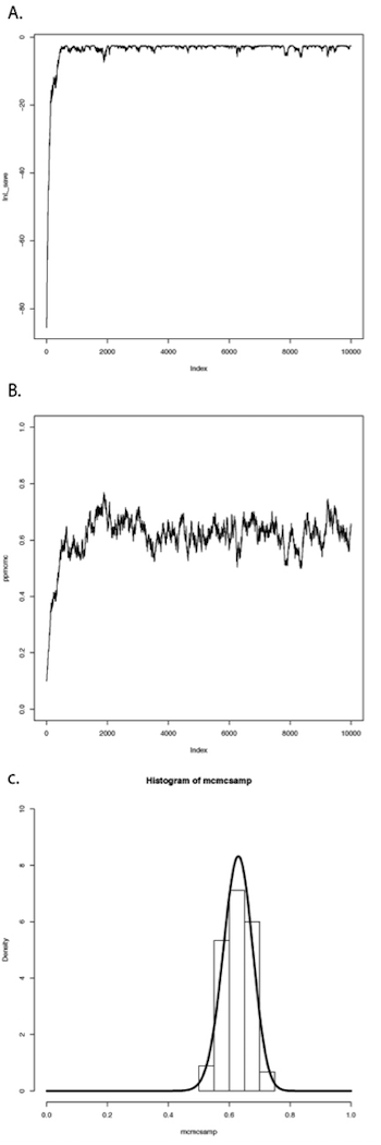
Figure 2.4. Bayesian MCMC from lizard flipping example. Image by the author, can be reused under a CC-BY-4.0 license.
This simple example glosses over some of the details of MCMC algorithms, but we will get into those details later, and there are many other books that treat this topic in great depth (e.g. Christensen et al. 2010). The point is that we can solve some of the challenges involved in Bayesian statistics using numerical “tricks” like MCMC, that exploit the power of modern computers to fit models and estimate model parameters.
Section 2.4c: Bayes factors
Now that we know how to use data and a prior to calculate a posterior distribution, we can move to the topic of Bayesian model selection. We already learned one general method for model selection using AIC. We can also do model selection in a Bayesian framework. The simplest way is to calculate and then compare the posterior probabilities for a set of models under consideration. One can do this by calculating Bayes factors:
(eq. 2.32)
$$
B_{12} = \frac{Pr(D|H_1)}{Pr(D|H_2)}
$$
Bayes factors are ratios of the marginal likelihoods P(D|H) of two competing models. They represent the probability of the data averaged over the posterior distribution of parameter estimates. It is important to note that these marginal likelihoods are different from the likelihoods used above for AIC model comparison in an important way. With AIC and other related tests, we calculate the likelihoods for a given model and a particular set of parameter values – in the coin flipping example, the likelihood for model 2 when pH = 0.63. By contrast, Bayes factors’ marginal likelihoods give the probability of the data averaged over all possible parameter values for a model, weighted by their prior probability.
Because of the use of marginal likelihoods, Bayes factor allows us to do model selection in a way that accounts for uncertainty in our parameter estimates – again, though, at the cost of requiring explicit prior probabilities for all model parameters. Such comparisons can be quite different from likelihood ratio tests or comparisons of AICc scores. Bayes factors represent model comparisons that integrate over all possible parameter values rather than comparing the fit of models only at the parameter values that best fit the data. In other words, AICc scores compare the fit of two models given particular estimated values for all of the parameters in each of the models. By contrast, Bayes factors make a comparison between two models that accounts for uncertainty in their parameter estimates. This will make the biggest difference when some parameters of one or both models have relatively wide uncertainty. If all parameters can be estimated with precision, results from both approaches should be similar.
Calculation of Bayes factors can be quite complicated, requiring integration across probability distributions. In the case of our coin-flipping problem, we have already done that to obtain the beta distribution in equation 2.22. We can then calculate Bayes factors to compare the fit of two competing models. Let’s compare the two models for coin flipping considered above: model 1, where pH = 0.5, and model 2, where pH = 0.63. Then:
(eq. 2.33)
$$
\begin{array}{lcl}
Pr(D|H_1) &=& \binom{100}{63} 0.5^{0.63} (1-0.5)^{100-63} \\\
&=& 0.00270 \\\
Pr(D|H_2) &=& \int_{p=0}^{1} \binom{100}{63} p^{63} (1-p)^{100-63} \\\
&=& \binom{100}{63} \beta (38,64) \\\
&=& 0.0099 \\\
B_{12} &=& \frac{0.0099}{0.00270} \\\
&=& 3.67 \\\
\end{array}
$$
In the above example, β(x, y) is the Beta function. Our calculations show that the Bayes factor is 3.67 in favor of model 2 compared to model 1. This is typically interpreted as substantial (but not decisive) evidence in favor of model 2. Again, we can be reasonably confident that our lizard is not a fair flipper.
In the lizard flipping example we can calculate Bayes factors exactly because we know the solution to the integral in equation 2.33. However, if we don’t know how to solve this equation (a typical situation in comparative methods), we can still approximate Bayes factors from our MCMC runs. Methods to do this, including arrogance sampling and stepping stone models (Xie et al. 2011; Perrakis et al. 2014), are complex and beyond the scope of this book. However, one common method for approximating Bayes Factors involves calculating the harmonic mean of the likelihoods over the MCMC chain for each model. The ratio of these two likelihoods is then used as an approximation of the Bayes factor (Newton and Raftery 1994). Unfortunately, this method is extremely unreliable, and probably should never be used (see Neal 2008 for more details).
Section 2.5: AIC versus Bayes
Before I conclude this section, I want to highlight another difference in the way that AIC and Bayes approaches deal with model complexity. This relates to a subtle philosophical distinction that is controversial among statisticians themselves so I will only sketch out the main point; see a real statistics book like Burnham and Anderson (2003) or Gelman et al. (2013) for further details. When you compare Bayes factors, you assume that one of the models you are considering is actually the true model that generated your data, and calculate posterior probabilities based on that assumption. By contrast, AIC assumes that reality is more complex than any of your models, and you are trying to identify the model that most efficiently captures the information in your data. That is, even though both techniques are carrying out model selection, the basic philosophy of how these models are being considered is very different: choosing the best of several simplified models of reality, or choosing the correct model from a set of alternatives.
The debate between Bayesian and likelihood-based approaches often centers around the use of priors in Bayesian statistics, but the distinction between models and “reality” is also important. More specifically, it is hard to imagine a case in comparative biology where one would be justified in the Bayesian assumption that one has identified the true model that generated the data. This also explains why AIC-based approaches typically select more complex models than Bayesian approaches. In an AIC framework, one assumes that reality is very complex and that models are approximations; the goal is to figure out how much added model complexity is required to efficiently explain the data. In cases where the data are actually generated under a very simple model, AIC may err in favor of overly complex models. By contrast, Bayesian analyses assume that one of the models being considered is correct. This type of analysis will typically behave appropriately when the data are generated under a simple model, but may be unpredictable when data are generated by processes that are not considered by any of the models. However, Bayesian methods account for uncertainty much better than AIC methods, and uncertainty is a fundamental aspect of phylogenetic comparative methods.
In summary, Bayesian approaches are useful tools for comparative biology, especially when combined with MCMC computational techniques. They require specification of a prior distribution and assume that the “true” model is among those being considered, both of which can be drawbacks in some situations. A Bayesian framework also allows us to much more easily account for phylogenetic uncertainty in comparative analysis. Many comparative biologists are pragmatic, and use whatever methods are available to analyze their data. This is a reasonable approach but one should remember the assumptions that underlie any statistical result.
Section 2.6: Models and comparative methods
For the rest of this book I will introduce several models that can be applied to evolutionary data. I will discuss how to simulate evolutionary processes under these models, how to compare data to these models, and how to use model selection to discriminate amongst them. In each section, I will describe standard statistical tests (when available) along with ML and Bayesian approaches.
One theme in the book is that I emphasize fitting models to data and estimating parameters. I think that this approach is very useful for the future of the field of comparative statistics for three main reasons. First, it is flexible; one can easily compare a wide range of competing models to your data. Second, it is extendable; one can create new models and automatically fit them into a preexisting framework for data analysis. Finally, it is powerful; a model fitting approach allows us to construct comparative tests that relate directly to particular biological hypotheses.
Footnotes
1: I assume here that you have little interest in organisms other than lizards.
2: And, often, concludes that we just "need more data" to get the answer that we want.
3: Especially in fields like genomics where multiple testing and massive Bonferroni corrections are common; one can only wonder at the legions of type II errors that are made under such circumstances.
References
Akaike, H. 1998. Information theory and an extension of the maximum likelihood principle. Pp. 199–213 in E. Parzen, K. Tanabe, and G. Kitagawa, eds. Selected papers of Hirotugu Akaike. Springer New York, New York, NY.
Burnham, K. P., and D. R. Anderson. 2003. Model selection and multimodel inference: A practical information theoretic approach. Springer Science & Business Media.
Edwards, A. W. F. 1992. Likelihood. Johns Hopkins University Press, Baltimore.
Gelman, A., J. B. Carlin, H. S. Stern, D. B. Dunson, A. Vehtari, and D. B. Rubin. 2013. Bayesian data analysis, third edition. Chapman; Hall/CRC.
Neal, R. 2008. The harmonic mean of the likelihood: Worst Monte Carlo method ever. Radford Neal’s blog.
Newton, M. A., and A. E. Raftery. 1994. Approximate Bayesian inference with the weighted likelihood bootstrap. J. R. Stat. Soc. Series B Stat. Methodol. 56:3–48.
Perneger, T. V. 1998. What’s wrong with Bonferroni adjustments. BMJ 316:1236–1238.
Perrakis, K., I. Ntzoufras, and E. G. Tsionas. 2014. On the use of marginal posteriors in marginal likelihood estimation via importance sampling. Comput. Stat. Data Anal. 77:54–69.
Posada, D., and K. A. Crandall. 1998. MODELTEST: Testing the model of DNA substitution. Bioinformatics 14:817–818.
Xie, W., P. O. Lewis, Y. Fan, L. Kuo, and M.-H. Chen. 2011. Improving marginal likelihood estimation for Bayesian phylogenetic model selection. Syst. Biol. 60:150–160.