Phylogenetic Comparative Methods learning from trees
- Chapter 8: Fitting models of discrete character evolution
- Section 8.1: The evolution of limbs and limblessness
- Section 8.2: Fitting Mk models to comparative data
- Section 8.3: Using maximum likelihood to estimate parameters of the Mk model
- Section 8.4: Using Bayesian MCMC to estimate parameters of the Mk model
- Section 8.5: Exploring Mk: the "total garbage" test
- Section 8.6: Testing for differences in the forwards and backwards rate of character change
- Section 8.7: Chapter summary
pdf version R markdown to recreate analyses
Chapter 8: Fitting models of discrete character evolution
Section 8.1: The evolution of limbs and limblessness
In the introduction to Chapter 7, I mentioned that squamates had lost their limbs repeatedly over their evolutionary history. This is a pattern that has been known for decades, but analyses have been limited by the lack of a large, well-supported species-level phylogenetic tree of squamates (but see Brandley et al. 2008). Only in the past few years have phylogenetic trees been produced at a scale broad enough to take a comprehensive look at this question [e.g. Bergmann and Irschick (2012); Pyron et al. (2013); see Figure 8.1]. Such efforts to reconstruct this section of the tree of life provide exciting potential to revisit old questions with new data.
![Figure 8.1. A view of the squamate tree of life. Data from Bergmann et al. (2012), visualized using OneZoom [Rosindell and Harmon (2012); see www.onezoom.org]. This image can be reused under a CC-BY-4.0 license.](/pcm/images/figure8-1.png)
Figure 8.1. A view of the squamate tree of life. Data from Bergmann et al. (2012), visualized using OneZoom [Rosindell and Harmon (2012); see www.onezoom.org]. This image can be reused under a CC-BY-4.0 license.
Plotting the pattern of limbed and limbless species on the tree leads to interesting questions about the tempo and mode of this trait in squamates. For example, are there multiple gains as well as losses of limbs? Do gains and losses happen at the same rate, or (as we might expect) are gains more rare than losses? We can test hypothesis such as these using the the Mk and extended-Mk models (see chapter 7). In this chapter we will fit these models to phylogenetic comparative data.
Section 8.2: Fitting Mk models to comparative data
The equations in Chapter 7 give us enough information to calculate the likelihood for comparative data on a tree. To understand how this is done, we can first consider the simplest case, where we know the beginning state of a character, the branch length, and the end state. We can then apply the method across an entire tree using a pruning algorithm, which will allow calculation of the likelihood of the data given the model and phylogenetic tree.
Imagine that a two-state character changes from a state of 0 to a state of 1 sometime over a time interval of t = 3. What is the likelihood of these data under the Mk model? As we did in equation 7.17, we can set a rate parameter q = 0.5 to calculate a probability matrix:
(eq. 8.1)
$$
\mathbf{P}(t) = e^{\mathbf{Q} t} = exp(
\begin{bmatrix}
-0.5 & 0.5 \\
0.5 & -0.5 \\
\end{bmatrix}
\cdot 3) =
\begin{bmatrix}
0.525 & 0.475 \\
0.475 & 0.525 \\
\end{bmatrix}
$$
For this simple example, we started with state 0, so we look at the first row. Along this branch, we ended at state 1, so we should look specifically at p12(t): the probability of starting with state 0 and ending with state 1 over time t. This value is the probability of obtaining the data given the model (i.e. the likelihood): L = 0.475.
This likelihood applies to the evolutionary process along this single branch.
When we have comparative data the situation is more complex. If we knew the ancestral character states and states at every node in the tree, then calculation of the overall likelihood would be straightforward – we could just apply the approach above many times, once for each branch of the tree. However, there are two problems. First, we don’t know the starting state of the character at the root of the tree, and must treat that as an unknown. Second, we are modeling a process that is happening independently on many branches in a phylogenetic tree, and only observe the states at the end of these branches. All of the character states at internal nodes of the tree are unknown. The likelihood that we want to calculate has to be summed across all of these unknown character state possibilities on the internal branches of the tree.
Thankfully, Felsenstein (1973) provides an elegant algorithm for calculating the likelihoods for discrete characters on a tree. This algorithm, called Felsenstein’s pruning algorithm, is described with an example in the appendix to this chapter. Felsenstein’s pruning algorithm was important in the history of phylogenetics because it allowed scientists to efficiently calculate the likelihoods of comparative data given a tree and a model. One can then maximize that likelihood by changing model parameters (and perhaps also the topology and branch lengths of the tree; see Felsenstein 2004).
Pruning also gives some insight into how we can calculate probabilities on trees; many other problems in comparative methods can be approached using different pruning algorithms.
Felsenstein’s pruning algorithm proceeds backwards in time from the tips to the root of the tree (see appendix, section 8.8). At the root, we must specify the probabilities of each character state in the common ancestor of the species in the clade. As mentioned in Chapter 7, there are at least three possible methods for doing this. First, one can assume that each state can occur at the root with equal probability. Second, one can assume that the states are drawn from their stationary distribution, as given by the model. The stationary distribution is a stable probability distribution of states that is reached by the model after a long amount of time. Third, one might have some information about the root state – perhaps from fossils, or information about character states in a set of outgroup taxa – that can be used to assign probabilities to the states. In practice, the first two of these methods are more common. In the case discussed above – an Mk model with all transition rates equal – the stationary distribution is one where all states are equally probable, so the first two methods are identical. In general, though, these three methods can give different results.
Section 8.3: Using maximum likelihood to estimate parameters of the Mk model
The algorithm in the appendix below gives the likelihood for any particular discrete-state Markov model on a tree, but requires us to specify a value of the rate parameter q. In the example given, this rate parameter q = 1.0 corresponds to a lnL of -6.5. But is this the best value of q to use for our Mk model? Probably not. We can use maximum likelihood to find a better estimate of this parameter.
If we apply the pruning algorithm across a range of different values of q, the likelihood changes. To find the ML estimate of q, we can again use numerical optimization methods, calculating the likelihood by pruning for many values of q and finding the maximum.
Applying this method to the lizard data, we obtain a maximum liklihood estimate of q = 0.001850204 corresponding to lnL = −80.487176.
The example above considers maximization of a single parameter, which is a relatively simple problem. When we extend this to a multi-parameter model – for example, the extended Mk model will all rates different (ARD) – maximizing the likelihood becomes much more difficult. R packages solve this problem by using sophisticated algorithms and applying them multiple times to make sure that the value found is actually a maximum.
Section 8.4: Using Bayesian MCMC to estimate parameters of the Mk model
We can also analyze this model using a Bayesian MCMC framework. We can modify the standard approach to Bayesian MCMC (see chapter 2):
Sample a starting parameter value, q, from its prior distributions. For this example, we can set our prior distribution as uniform between 0 and 1. (Note that one could also treat probabilities of states at the root as a parameter to be estimated from the data; in this case we will assign equal probabilities to each state).
Given the current parameter value, select new proposed parameter values using the proposal density Q(q′|q). For example, we might use a uniform proposal density with width 0.2, so that Q(q′|q) U(q − 0.1, q + 0.1).
Calculate three ratios:
a. The prior odds ratio, Rprior. In this case, since our prior is uniform, Rprior = 1.
b. The proposal density ratio, Rproposal. In this case our proposal density is symmetrical, so Rproposal = 1.
c. The likelihood ratio, Rlikelihood. We can calculate the likelihoods using Felsenstein’s pruning algorithm (Box 8.1); then calculate this value based on equation 2.26.
Find Raccept as the product of the prior odds, proposal density ratio, and the likelihood ratio. In this case, both the prior odds and proposal density ratios are 1, so Raccept = Rlikelihood
Draw a random number u from a uniform distribution between 0 and 1. If u < Raccept, accept the proposed value of both parameters; otherwise reject, and retain the current value of the two parameters.
Repeat steps 2-5 a large number of times.
We can run this analysis on our squamate data, obtaining a posterior with a mean estimate of q = 0.001980785 and a 95% credible interval of 0.001174813 − 0.003012715.
Section 8.5: Exploring Mk: the "total garbage" test
One problem that arises sometimes in maximum likelihood optimization happens when instead of a peak, the likelihood surface has a long flat “ridge” of equally likely parameter values. In the case of the Mk model, it is common to find that all values of q greater than a certain value have the same likelihood. This is because above a certain rate, evolution has been so rapid that all traces of the history of evolution of that character have been obliterated. After this point, character states of each lineage are random, and have no relationship to the shape of the phylogenetic tree. Our optimization techniques will not work in this case because there is no value of q that has a higher likelihood than other values. Once we get onto the ridge, all values of q have the same likelihood.
For Mk models, there is a simple test that allows us to recognize when the likelihood surface has a long ridge, and q values cannot be estimated. I like to call this test the “total garbage” test because it can tell you if your data are “garbage” with respect to historical inference – that is, your data have no information about historical patterns of trait change. One can predict states just as well by choosing each species at random.
To carry out the total garbage test, imagine that you are just drawing trait values at random. That is, each species has some probability p of having character state 0, and some probability (1 − p) of having state 1 (one can also generalize this test to multi-state models). This likelihood is easy to write down. For a tree of size n, the probability of drawing n0 species with state 0 is:
(eq. 8.2)
Lgarbage = pn0(1 − p)n − n0
This equation gives the likelihood of the “total garbage” model for any value of p. Equation 8.1 is related to a binomial distribution (lacking only the factorial term). We also know from probability theory that the ML estimate of p is n0/n, with likelihood given by the above formula.
Now consider the likelihood surface of the Mk model. When Mk likelihood surfaces have long ridges, they are nearly always for high values of q – and when the transition rate of character changes is high, this model converges to our “drawing from a hat” (or “garbage”) model. The likelihood ridge lies at the value that is exactly taken from equation 8.10 above.
Thus, one can compare the likelihood of our Mk model to the total garbage model. If the maximum likelihood value of q has the same likelihood as our garbage model, then we know that we are on a ridge of the likelihood surface and q cannot be estimated. We also have no ability to make any statements about the past evolution of our character – in particular, we cannot estimate ancestral character state with any precision. By contrast, if the likelihood of the Mk model is greater than the total garbage model, then our data contains some historical information. We can also make this comparison using AIC, considering the total garbage model as having a single parameter p.
For the squamates, we have n = 258 and n0 = 207. We calculate p = n0/n = 207/258 = 0.8023256. So the likelihood of our garbage model is Lgarbage = pn0(1 − p)n − n0 = 0.8023256207(1 − 0.8023256)51 = 1.968142e − 56. This calculation is both easier and more useful, though, on a natural-log scale: lnLgarbage = n0 ⋅ ln(p)+(n − n0)⋅ln(1 − p)=207 ⋅ ln(0.8023256)+51 ⋅ ln(1 − 0.8023256)= − 128.2677. Compare this to the log-likelihood of our Mk model, lnL = −80.487176, and you will see that the garbage model is a terrible fit to these data. There is, in fact, some historical information about species' traits in our data.
Section 8.6: Testing for differences in the forwards and backwards rate of character change
I have been referring to an example of lizard limb evolution throughout this chapter, but we have not yet tested the hypothesis that I stated in the introduction: that transition rates for losing limbs are higher than rates of gaining limbs.
To do this, we can compare our one-rate Mk model with a two-rate model with differences in the rate of forwards and backwards transitions. The character states are 1 (no limbs) and 2 (limbs), and the forward transition represents gaining limbs. This is a special case of the “all-rates different” model discussed in chapter two. Q matrices for these two models will be, for model 1 (equal rates):
(eq. 8.3)
$$
\mathbf{Q_{ER}} =
\begin{bmatrix}
-q & q \\
q & -q \\
\end{bmatrix}
$$
$$
\mathbf{\pi_{ER}} =
\begin{bmatrix}
1/2 & 1/2 \\
\end{bmatrix}
$$
And for model 2, asymmetric:
(eq. 8.4)
$$
\mathbf{Q_{ASY}} =
\begin{bmatrix}
-q_1 & q_1 \\
q_2 & -q_2 \\
\end{bmatrix}
$$
$$
\mathbf{\pi_{ASY}} =
\begin{bmatrix}
1/2 & 1/2 \\
\end{bmatrix}
$$
Notice that the ER model has one parameter, while the ASY model has two. Also we have specified equal probabilities of each character at the root of the tree, which may not be justified. But this comparison is still useful as a simple example.
One can compare the two nested models using standard methods discussed in previous chapters – that is, a likelihood-ratio test, AIC, BIC, or other similar methods.
We can apply all of the above methods to analyze the evolution of limblessness in squamates. We can use the tree and character state data from Brandley et al. (2008), which is plotted with ancestral state reconstructions under an ER model in Figure 8.2.
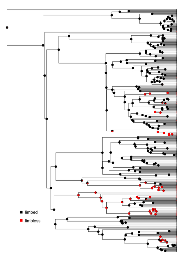
Figure 8.2. Reconstructed patterns of the evolution of limbs and limblessness across squamates. Tips show states of extant taxa (here, I classified species with neither fore- nor hindlimbs as limbless, which is conservative given the variation across this clade (see chapter 7). Pie charts on internal nodes show proportional marginal likelihoods for ancestral state reconstruction under an ER model. Data from Brandley et al. (2008). Image by the author, can be reused under a CC-BY-4.0 license.
If we fit an Mk model to these data assuming equal state frequencies at the root of the tree, we obtain a lnL of -80.5 and an estimate of the QER matrix as:
(eq. 8.5)
$$
\mathbf{Q_{ER}} =
\begin{bmatrix}
-0.0019 & 0.0019 \\
0.0019 & -0.0019 \\
\end{bmatrix}
$$
The ASY model with different forward and backward rates gives a lnL of -79.4 and:
(eq. 8.6)
$$
\mathbf{Q_{ASY}} =
\begin{bmatrix}
-0.0016 & 0.0016 \\
0.0038 & -0.0038 \\
\end{bmatrix}
$$
Note that the ASY model has a higher backwards than forwards rate; as expected, we estimate a rate of losing limbs that is higher than the rate of gaining them (although the difference is surprisingly low). Is this statistically supported? We can compare the AIC scores of the two models. For the ER model, AICc = 163.0, while for the ASY model AICc = 162.8. The AICc score is higher for the unequal rates model, but only by about 0.2 – which is not definitive either way. So based on this analysis, we cannot rule out the possibility that forward and backward rates are equal.
A Bayesian analysis of the ASY model gives similar conclusions (Figure 8.3). We can see that the posterior distribution for the backwards rate (q21) is higher than the forwards rate (q12), but that the two distributions are broadly overlapping.
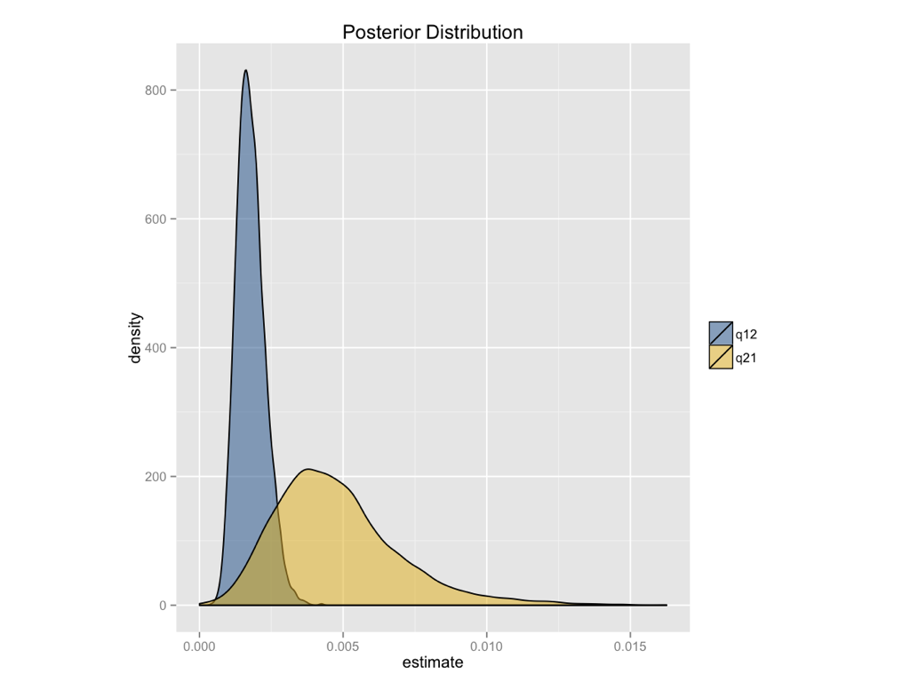
Figure 8.3. Bayesian posterior distibutions for the extended-Mk model applied to the evolution of limblessness in squamates. Image by the author, can be reused under a CC-BY-4.0 license.
You might wonder about how we can reconcile these results, which suggest that squamates gain limbs at least as frequently as they lose them, with our biological intuition that limbs should be much more difficult to gain than they are to lose. But keep in mind that our comparative analysis is not using any information other than the states of extant species to reconstruct these rates. In particular, identifying irreversible evolution using comparative methods is a problem that is known to be quite difficult, and might require outside information in order to resolve conclusively. For example, if we had some information about the relative number of mutational steps required to gain and lose limbs, we could use an informative prior – which would, I suspect, suggest that limbs are more difficult to gain than they are to lose. Such a prior could dramatically alter the results presented in Figure 8.3. We will return to the problem of irreversible evolution later in the book (Chapter 13).
Section 8.7: Chapter summary
In this chapter I describe how Felsenstein’s pruning algorithm can be used to calculate the likelihoods of Mk and extended-Mk models on phylogenetic trees. I have also described both ML and Bayesian frameworks that can be used to test hypotheses about character evolution. This chapter also includes a description of the “total garbage” test, which will tell you if your data has information about evolutionary rates of a given character.
Analyzing our example of lizard limbs shows the power of this approach; we can estimate transition rates for this character over macroevolutionary time, and we can say with some certainty that transitions between limbed and limbless have been asymmetric. In the next chapter, we will build on the Mk model and further develop our comparative toolkit for understanding the evolution of discrete characters.
Section 8.8: Appendix: Felsenstein's pruning algorithm
Felsenstein’s pruning algorithm (1973) is an example of dynamic programming, a type of algorithm that has many applications in comparative biology. In dynamic programming, we break down a complex problem into a series of simpler steps that have a nested structure. This allows us to reuse computations in an efficient way and speeds up the time required to make calculations.
The best way to illustrate Felsenstein’s algorithm is through an example, which is presented in the panels below. We are trying to calculate the likelihood for a three-state character on a phylogenetic tree that includes six species.
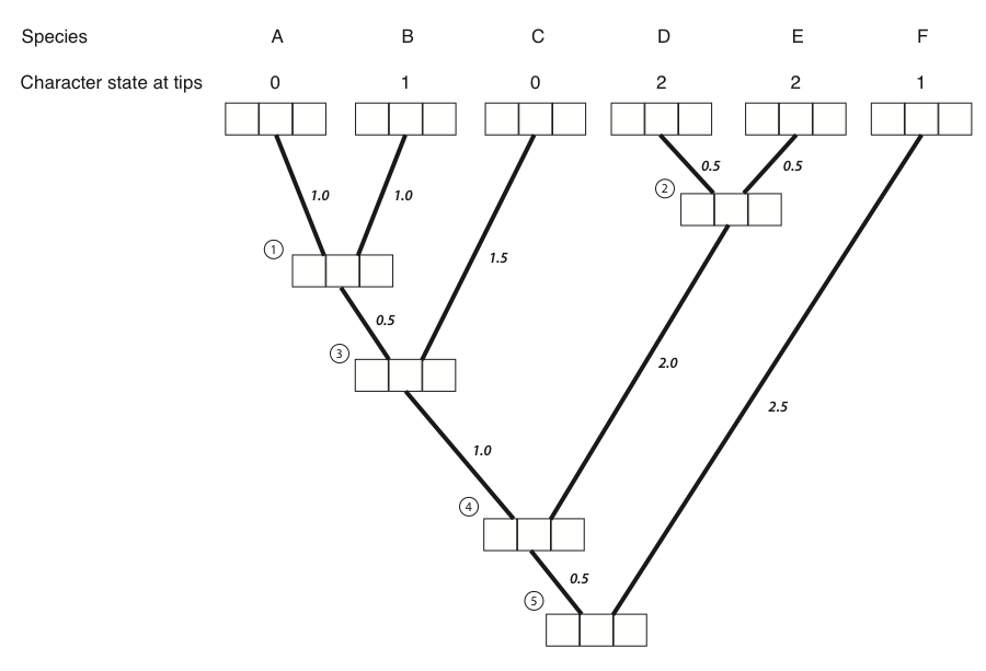
Figure 8.4A. Each tip and internal node in the tree has three boxes, which will contain the probabilities for the three character states at that point in the tree. The first box represents a state of 0, the second state 1, and the third state 2. Image by the author, can be reused under a CC-BY-4.0 license.
- The first step in the algorithm is to fill in the probabilities for the tips. In this case, we know the states at the tips of the tree. Mathematically, we state that we know precisely the character states at the tips; the probability that that species has the state that we observe is 1, and all other states have probability zero:

Figure 8.4B. We put a one in the box that corresponds to the actual character state and zeros in all others. Image by the author, can be reused under a CC-BY-4.0 license.
Next, we identify a node where all of its immediate descendants are tips. There will always be at least one such node; often, there will be more than one, in which case we will arbitrarily choose one. For this example, we will choose the node that is the most recent common ancestor of species A and B, labeled as node 1 in Figure 8.2B.
We then use equation 7.6 to calculate the conditional likelihood for each character state for the subtree that includes the node we chose in step 2 and its tip descendants. For each character state, the conditional likelihood is the probability, given the data and the model, of obtaining the tip character states if you start with that character state at the root. In other words, we keep track of the likelihood for the tipward parts of the tree, including our data, if the node we are considering had each of the possible character states. This calculation is:
$$
L_P(i) = (\sum\limits_{x \in k}Pr(x|i,t_L)L_L(x)) \cdot (\sum\limits_{x \in k}Pr(x|i,t_R)L_R(x))
$$
Where i and x are both indices for the k character states, with sums taken across all possible states at the branch tips (x), and terms calculated for each possible state at the node (i). The two pieces of the equation are the left and right descendant of the node of interest. Branches can be assigned as left or right arbitrarily without affecting the final outcome, and the approach also works for polytomies (but the equation is slightly different). Furthermore, each of these two pieces itself has two parts: the probability of starting and ending with each state along the two branches being considered, and the current conditional likelihoods that enter the equation at the tips of the subtree (LL(x) and LR(x)). Branch lengths are denoted as tL and tR for the left and right, respectively.
One can think of the likelihood "flowing" down the branches of the tree, and conditional likelihoods for the left and right branches get combined via multiplication at each node, generating the conditional likelihood for the parent node for each character state (LP(i)).
Consider the subtree leading to species A and B in the example given. The two tip character states are 0 (for species A) and 1 (for species B). We can calculate the conditional likelihood for character state 0 at node 1 as:
(eq. 8.8)
$$
L_P(0) = (\sum\limits_{x \in k}Pr(x|0,t_L=1.0)L_L(x)) \cdot (\sum\limits_{x \in k}Pr(x|0,t_R=1.0)L_R(x))
$$
Next, we can calculate the probability terms from the probability matrix P. In this case tL = tR = 1.0, so for both the left and right branch:
(eq. 8.9)
$$
\mathbf{Q}t =
\begin{bmatrix}
-2 & 1 & 1 \\
1 & -2 & 1 \\
1 & 1 & -2 \\
\end{bmatrix} \cdot 1.0 =
\begin{bmatrix}
-2 & 1 & 1 \\
1 & -2 & 1 \\
1 & 1 & -2 \\
\end{bmatrix}
$$
$$
\mathbf{P} = e^{Qt} =
\begin{bmatrix}
0.37 & 0.32 & 0.32 \\
0.32 & 0.37 & 0.32 \\
0.32 & 0.32 & 0.37 \\
\end{bmatrix}
$$
Now notice that, since the left character state is known to be zero, LL(0)=1 and LL(1)=LL(2)=0. Similarly, the right state is one, so LR(1)=1 and LR(0)=LR(2)=0.
We can now fill in the two parts of equation 8.2:
(eq. 8.11)
$$
\sum\limits_{x \in k}Pr(x|0,t_L=1.0)L_L(x) = 0.37 \cdot 1 + 0.32 \cdot 0 + 0.32 \cdot 0 = 0.37
$$
$$
\sum\limits_{x \in k}Pr(x|0,t_R=1.0)L_R(x) = 0.37 \cdot 0 + 0.32 \cdot 1 + 0.32 \cdot 0 = 0.32
$$
LP(0)=0.37 ⋅ 0.32 = 0.12.
This means that under the model, if the state at node 1 were 0, we would have a likelihood of 0.12 for this small section of the tree. We can use a similar approach to find that:
(eq. 8.13)
LP(1)=0.32 ⋅ 0.37 = 0.12.
LP(2)=0.32 ⋅ 0.32 = 0.10.
Now we have the likelihood for all three possible ancestral states. These numbers can be entered into the appropriate boxes:

Figure 8.4C. Conditional likelihoods entered for node 1. Image by the author, can be reused under a CC-BY-4.0 license.
- We then repeat the above calculation for every node in the tree. For nodes 3-5, not all of the LL(x) and LR(x) terms are zero; their values can be read out of the boxes on the tree. The result of all of these calculations:

Figure 8.4D. Conditional likelihoods entered for all nodes. Image by the author, can be reused under a CC-BY-4.0 license.
- We can now calculate the likelihood across the whole tree using the conditional likelihoods for the three states at the root of the tree.
$$
L = \sum\limits_{x \in k} \pi_x L_{root} (x)
$$
Where πx is the prior probability of that character state at the root of the tree. For this example, we will take these prior probabilities to be uniform, equal for each state (πx = 1/k = 1/3). The likelihood for our example, then, is:
(eq. 8.15)
L = 1/3 ⋅ 0.00150 + 1/3 ⋅ 0.00151 + 1/3 ⋅ 0.00150 = 0.00150
Note that if you try this example in another software package, like GEIGER or PAUP*, the software will calculate a ln-likelihood of -6.5, which is exactly the natural log of the value calculated here.
References
Bergmann, P. J., and D. J. Irschick. 2012. Vertebral evolution and the diversification of squamate reptiles. Evolution 66:1044–1058. Wiley Online Library.
Brandley, M. C., J. P. Huelsenbeck, and J. J. Wiens. 2008. Rates and patterns in the evolution of snake-like body form in squamate reptiles: Evidence for repeated re-evolution of lost digits and long-term persistence of intermediate body forms. Evolution. Wiley Online Library.
Felsenstein, J. 2004. Inferring phylogenies. Sinauer Associates, Inc., Sunderland, MA.
Felsenstein, J. 1973. Maximum likelihood and minimum steps methods for estimating evolutionary trees from data on discrete characters. Syst. Biol. 22:240–249. Oxford University Press.
Pyron, R. A., F. T. Burbrink, and J. J. Wiens. 2013. A phylogeny and revised classification of squamata, including 4161 species of lizards and snakes. BMC Evol. Biol. 13:93. bmcevolbiol.biomedcentral.com.
Rosindell, J., and L. J. Harmon. 2012. OneZoom: A fractal explorer for the tree of life. PLoS Biol. 10:e1001406.