Phylogenetic Comparative Methods learning from trees
Chapter 12: Beyond birth-death models
Section 12.1: Capturing variable evolution
As we discovered in Chapter 11, there are times and places where the tree of life has grown more rapidly than others. For example, islands and island-like habitats are sometimes described as hotspots of speciation (Losos and Schluter 2000; Hughes and Eastwood 2006), and diversification rates in such habitats can proceed at an extremely rapid pace. On a broader scale, many studies have shown that speciation rates are elevated and/or extinction rates depressed following mass extinctions (e.g. Sepkoski 1984). Finally, some clades seem to diversity much more rapidly than others. In my corner of the world, the Pacific Northwest of the United States, this variation is best seen in our local amphibians. We have species like the spotted frog and the Pacific tree frog, which represent two very diverse frog lineages with high diversification rates (Ranidae and Hylidae, respectively; Roelants et al. 2007). At the same time, if one drives a bit to the high mountain streams, you can find frogs with tiny tails. These Inland Tailed Frogs are members of Ascaphidae, a genus with only two species, one coastal and one inland. (As an aside, the tail, found only in males, is an intromittent organ used for internal fertilization - analogous to a penis, but different!) These two tailed frog species are the sister group to a small radiation of four species frogs in New Zealand (Leopelmatidae, which have no tails). These two clades together - just six species - make up the sister clade to all other frogs, nearly 7000 species (Roelants et al. 2007; Jetz and Pyron 2018). We seek to explain patterns like this contrast in the diversity of two groups which decend from a common ancestor and are, thus, the same age.
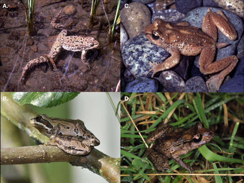
Figure 12.1. Contrasts in frog diversity. Spotted frogs (A) and Pacific tree frogs (B) come from diverse clades, while tailed frogs (C) and New Zealand frogs (D) are from depauperate clades. Photo credits: A: Sean Neilsen / Wikimedia Commons / Public Domain, B: User:The High Fin Sperm Whale / Wikimedia Commons / CC-BY-SA-3.0, C: User:Leone.baraldi / Wikimedia Commons / CC-BY-SA-4.0, D: Phil Bishop / Wikimedia Commons / CC-BY-SA-2.5.
Simple, constant-rate birth-death models are not adequate to capture the complexity and dynamics of speciation and extinction across the tree of life. Speciation and extinction rates vary through time, across clades, and among geographic regions. We can sometimes predict this variation based on what we know about the mechanisms that lead to speciation and/or extinction.
In this chapter, I will explore some extensions to birth-death models that allow us to explore diversification in more detail. This chapter also leads naturally to the next, chapter 13, which will consider the case where diversification rates depend on species’ traits.
Section 12.2: Variation in diversification rates across clades
We know from analyses of tree balance that the tree of life is more imbalanced than birth-death models predict. We can explore this variation in diversification rates by allowing birth and death models to vary along branches in phylogenetic trees. The simplest scenario is when one has a particular prediction about diversification rates to test. For example, we might wonder if diversification rates in one clade (clade A in Figure 12.2) are higher than in the rest of the phylogenetic tree. We can test this hypothesis by fitting a multiple-rate birth-death model.
The simplest method to carry out this test is by using model selection in a ML framework (Rabosky et al. 2007). To do this, we first fit a constant-rates birth-death model to the entire tree, and calculate a likelihood. We can then fit variable-rates birth-death models to the data, comparing the fit of these models using either likelihood ratio tests or AICC. The simplest way to fit a variable-rates model is to adapt the likelihood formula in equation 11.18 (or eq. 11.24 if species are unsampled). We calculate the likelihood in two parts, one for the background part of the tree (with rates λB and μB) and one for the focal clade that may have different diversification dynamics (with rates λA and μA). We can then compare this model to one where speciation and extinction rates are constant through time.
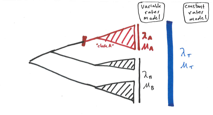
Figure 12.2. A phylogenetic tree including three clades, illustrating two possible models for diversification: a constant rates model, where all three clades have the same diversification parameters λT and μT, and a variable rates model, where clade A has parameters (λA and μA) that differ from those of the other two clades (λB and μB). Image by the author, can be reused under a CC-BY-4.0 license.
Consider the example in Figure 12.2. We would like to know whether clade A has speciation and extinction rates, λA and μA, that differ from the background rates, λB and μB – we will call this a “variable rates” model. The alternative is a “constant rates” model where the entire clade has constant rate parameters λT and μT. These two models are nested, since the constant-rates model is a special case of the variable rates model where λT = λA = λB and μT = μA = μB. Calculating the likelihood for these two models is reasonably straightforward - we simply calculate the likelihood for each section of the tree using the relevant equation from Chapter 11, and then multiply the likelihoods from the two parts of the tree (or add the log-likelihoods) to get the overall likelihood.
For a real example, let’s look at the phylogenetic tree of amphibians and evaluate the hypothesis that the tailed and New Zealand frogs, sister clade to the rest of frogs, diversified at a slower rate than other amphibians (Figure 12.3). We can use the phylogenetic "backbone" tree from Jetz and Pyron (Jetz and Pyron 2018), assigning diversities based on the classification associated with that publication. We can then calculate likelihoods based on equation 11.24.
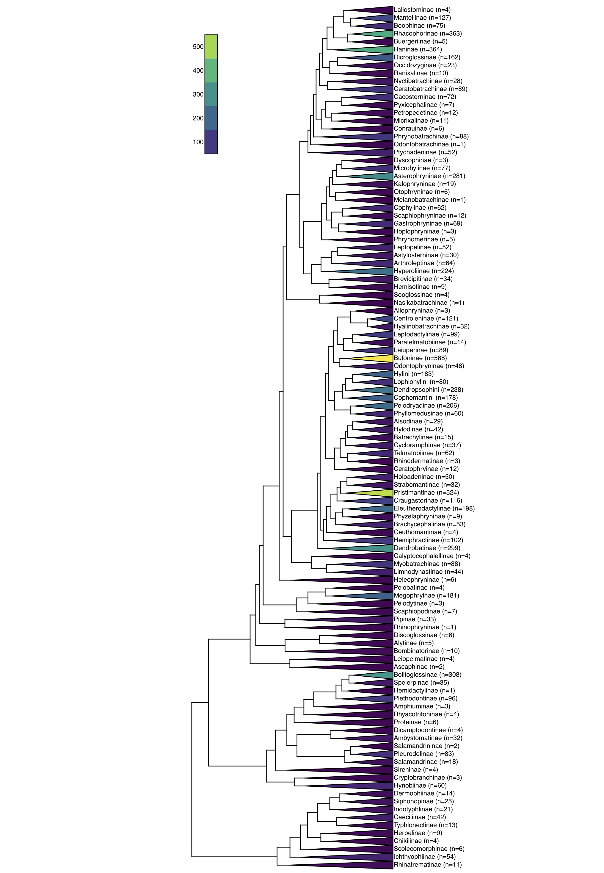
Figure 12.3. Phylogenetic tree of amphibians with divergence times and diversities of major clades. Data from Jetz and Pyron (Jetz and Pyron 2018). Image by the author, can be reused under a CC-BY-4.0 license.
We can calculate the likelihood of the constant rates model, with two parameters λT and μT, to a variable rates model with four parameters λliop, μliop, λother, and μother. For this example, we obtain the following results.
| Model | Parameter estimates | ln-Likelihood | AICc |
|---|---|---|---|
| Constant rates | λT = 0.30 | -1053.9 | 2111.8 |
| μT = 0.28 | |||
| Variable rates | lambdaliop = 0.010 | -1045.4 | 2101.1 |
| μliop = 0.007 | |||
| lambdaother = 0.29 | |||
| μother = 0.27 |
With a difference in AICc of more than 10, we see from these results that there is good reason to think that there is a difference in diversification rates in these "oddball" frogs compared to the rest of the amphibians.
Of course, more elaborate comparisons are possible. For example, one could compare the fit of four models, as follows: Model 1, constant rates; Model 2, speciation rate in clade A differs from the background; Model 3, extinction rate in clade A differs from the background; and Model 4, both speciation and extinction rates in clade A differ from the background. In this case, some of the pairs of models are nested – for example, Model 1 is a special case of Model 2, which is, in turn, a special case of Model 4 – but all four do not make a nested series. Here we benefit from using a model selection approach based on AICC. We can fit all four models and use their relative number of parameters to calculate AICC scores. We can then calculate AICC weights to evaluate the relative support for each of these four models. (As an aside, it might be difficult to differentiate among these four possibilities without a lot of data!)
But what if you do not have an a priori reason to predict differential diversification rates across clades? Or, what if the only reason you think one clade might have a different diversification rate than another is that it has more species? (Such reasoning is circular, and will wreak havoc with your analyses!) In such cases, we can use methods that allow us to fit general models where diversification rates are allowed to vary across clades in the tree. Available methods use stepwise AIC (MEDUSA, Alfaro et al. 2009; but see May and Moore 2016), or reversible-jump Bayesian MCMC (Rabosky 2014, 2017; but see Moore et al. 2016).
For example, running a stepwise-AIC algorithm on the amphibian data (Alfaro et al. 2009) results in a model with 11 different speciation and extinction regimes (Figure 12.4). This is good evidence that diversification rates have varied wildly through the history of amphibians.
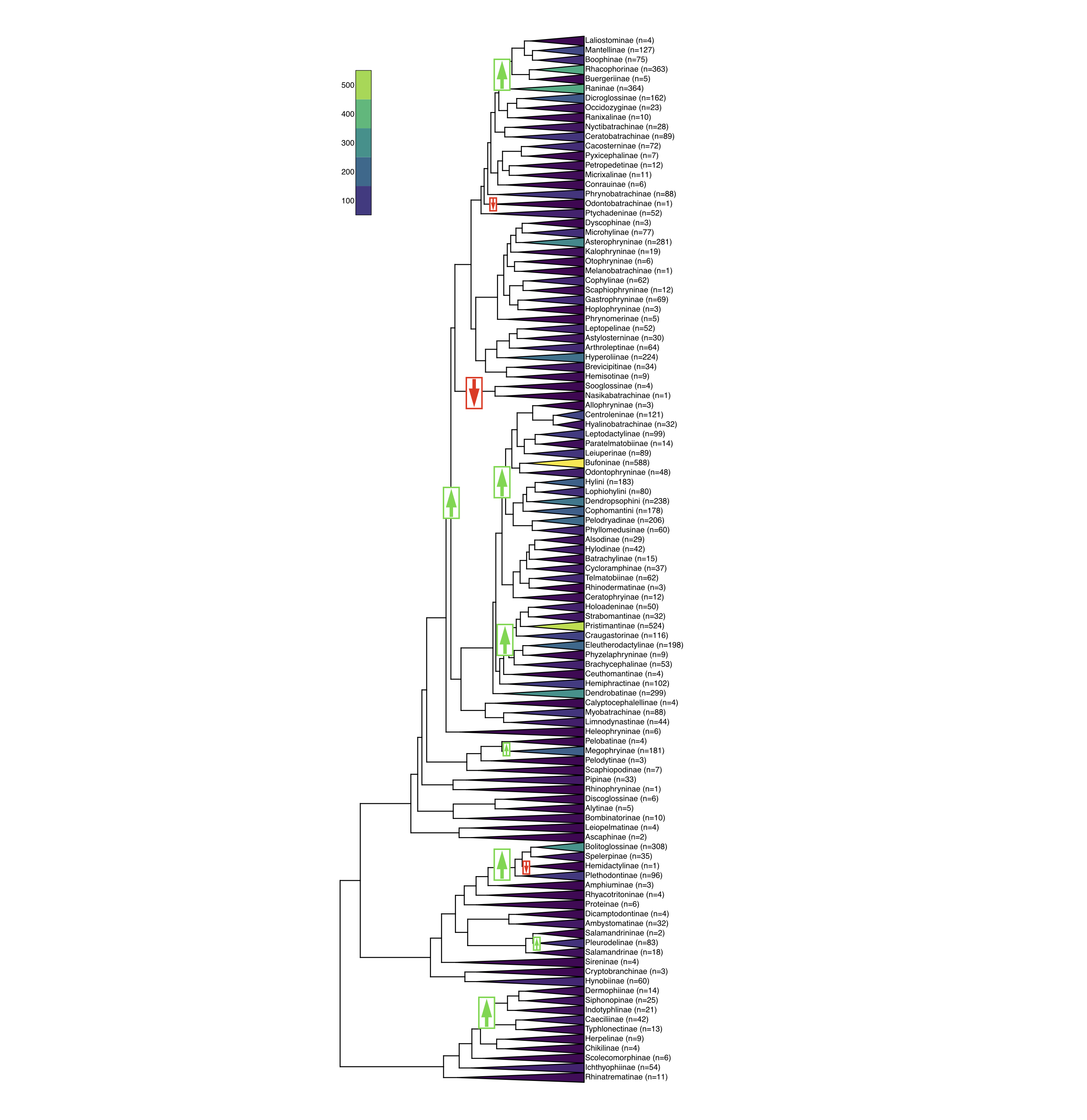
Figure 12.4. Analysis of diversification rate shifts among amphibian clades using MEDUSA (Alfaro et al. 2009). Arrows highlight places where speciation, extinction, or both are inferred to have shifted; green arrows indicate an inferred increase in r = λ − μ, while red arrows indicate decreased r. Data from Jetz and Pyron (Jetz and Pyron 2018). Image by the author, can be reused under a CC-BY-4.0 license.
One note: all current approaches fit a model where birth and death rates change at discrete times in the phylogenetic tree - that is, along certain branches in the tree leading to extant taxa. One might wish for an approach, then, that models such changes - using, for example, a Poisson process - and then locates the changes on the tree. However, we still lack the mathematics to solve for E(t) (e.g. equation 11.19) under such a model (Moore et al. 2016). Given that, we can view current implementations of models where rates vary across clades as an approximation to the likelihood, and one that discounts the possibility of shifts in speciation and/or extinction rates among any clades that did not happen to survive until the present day (Rabosky 2017) - and we are stuck with that until a better alternative is developed!
Section 12.3: Variation in diversification rates through time
In addition to considering rate variation across clades, we might also wonder whether birth and/or death rates have changed through time. For example, perhaps we think our clade is an adaptive radiation that experienced rapid diversification upon arrival to an island archipelago and slowed as this new adaptive zone got filled (Schluter 2000). This hypothesis is an example of density-dependent diversification, where diversification rate depends on the number of lineages that are present (Rabosky 2013). Alternatively, perhaps our clade has been experiencing extinction rates that have changed through time, perhaps peaking during some time period of unfavorable climactic conditions (Benton 2009). This is another hypothesis that predicts variation in diversification (speciation and extinction) rates through time.
We can fit time-dependent diversification models using likelihood equations that allow arbitrary variation in speciation and/or extinction rates, either as a function of time or depending on the number of other lineages in the clade. To figure out the likelihood we can first make a simplifying assumption: though diversification rates might change, they are constant across all lineages at any particular time point. In particular, this means that speciation (and/or extinction) rates slow down (or speed up) in exactly the same way across all lineages in an evolving clade. This is again the Equal-Rates Markov (ERM) model for tree growth described in the previous chapter.
Our assumption about equal rates across lineages at any time means that we can consider time-slices through the tree rather than individual branches, i.e. we can get all the information that we need to fit these models from lineage through time plots.
The most general way to fit time-varying birth-death models to phylogenetic trees is described in Morlon et al. (2011). Consider the case where both speciation and extinction rates vary as a function of time, λ(t) and μ(t). Morlon et al. (2011) derive the likelihood for such a model as:
(eq. 12.1)
$$
L(t_1, t_2, \dots, t_{n-1}) = (n+1)! \frac{f^n \sum_{i=1}^{n-1} \lambda(t_i) \Psi(s_{i,1}, t_i) \Psi(s_{i,2}, t_i)}{\lambda [1-E(t_1)]^2}
$$
Where:
(eq. 12.2)
$$
E(t) = 1 - \frac{e^{\int_0^t [\lambda(u) - \mu(u)]du}}{\frac{1}{f} + \int_0^t e^{\int_0^s [\lambda(u) - \mu(u)]du} \lambda(s) ds}
$$
and:
(eq. 12.3)
$$
\Psi(s, t) = e^{\int_s^t [\lambda(u) - \mu(u)]du} \Big[ 1 + \frac{\int_s^t e^{\int_0^\tau [\lambda(\sigma) - \mu(\sigma)]d\sigma}\lambda(\tau)d\tau}{\frac{1}{f} + \int_0^s e^{\int_0^\tau [\lambda(\sigma) - \mu(\sigma)]d\sigma} \lambda(\tau) d\tau} \Big]^{-2}
$$
Following chapter 11, n is the number of tips in the tree, and divergence times t1, t2, …, tn − 1 are defined as measured from the present (e.g. decreasing towards the present day). λ(t) and μ(t) are speciation and extinction rates expressed as an arbitrary function of time, f is the sampling fraction (under a uniform sampling model). For a node starting at time ti, si, 1 and si, 2 are the times when the two daughter lineages encounter a speciation event in the reconstructed tree1. E(t), as before, is the probability that a lineage alive at time t leaves no descendants in the sample. Finally, Ψ(s, t) is the probability that a lineage alive at time s leaves exactly one descent at time t < s in the reconstructed tree. These equations look complex, and they are - but basically involve integrating the speciation and extinction functions (and their difference) along the branches of the phylogenetic tree.
Note that my equations here differ from the originals in Morlon et al. (2011) in two ways. First, Morlon et al. (2011) assumed that we have information about the stem lineage and, thus, used an index on ti that goes up to n instead of n − 1 and a different denominator conditioning on survival of the descendants of the single stem lineage (Morlon et al. 2011). Second, I also multiply by the total number of topological arrangements of n taxa, (n + 1)!.
If one substitutes constants for speciation and extinction (λ(t)=λc, μ(t)=μc) in equation 12.1, then one obtains equation 11.24; if one additionally considers the case of complete sampling and substitutes f = 1 then we obtain equation 11.18. This provides a single unified framework for time-varying phylogenetic trees with uniform incomplete sampling (see also Höhna 2014 for independent but equivalent derivations that also extend to the case of representative sampling).
Equation 12.1 requires that we define speciation rate as a function of time. Two types of time-varying models are currently common in the comparative literature: linear and expoential. If speciation rates change linearly through time (see Rabosky and Lovette 2008 for an early version of this model):
(eq. 12.4)
λ(t)=λ0 + αλt
Where λ0 is the initial speciation rate at the present and alpha is the slope of speciation rate change as we go back through time. αλ must be chosen so that speciation rates do not become negative as we move back through the tree: αλ > −λ0/t1. Note that the interpretation of αλ is a bit strange since we measure time backwards: a positive αλ, for example, would mean that speciation rates have declined from the past to the present. Other time-dependent models published earlier (e.g. Rabosky and Lovette 2008, which considered a linearly declining pure-birth model) do not have this property.
We could also consider a linear change in extinction through time:
(eq. 12.5)
μ(t)=μ0 + αμt
Again, αμ is the change in extinction rate through time, and must be interpreted in the same "backwards" way as αλ. Again, we must restrict our parameter to avoid a negative rate: αμ > −μ0/t1
One can then substitute either of these formulas into equation 12.1 to calculate the likelihood of a model where speciation rate declines through time. Many implementations of this approach use numerical approximations rather than analytic solutions (see, e.g., Morlon et al. 2011; Etienne et al. 2012).
Another common model has speciation and/or extinction rates changing exponentially through time:
(eq. 12.6)
λ(t)=λ0eβλt
and/or
(eq. 12.7)
μ(t)=μ0eβμt
We can again calculate likelihoods for this model numerically (Morlon et al. 2011, Etienne et al. (2012)).
As an example, we can test models of time-varying diversification rates across part of the amphibian tree of life from Jetz and Pyron (2018). I will focus on one section of the salamanders, the lungless salamanders (Plethodontidae, comprised of the clade that spans Bolitoglossinae, Spelerpinae, Hemidactylinae, and Plethodontinae). This interesting clade was already identified above as including both an increase in diversification rates (at the base of the clade) and a decrease (on the branch leading to Hemidactylinae; Figure 12.4). The tree I am using may be missing a few species; this section of the tree includes 440 species in Jetz and Pyron (2018) but 471 speices are listed on Amphibiaweb as of May 2018. Thus, I will assume random sampling with f = 440/471 = 0.934.
Comparing the fit of a set of models, we obtain the following results:
| Model | Number of params. | Param. estimates | lnL | AIC |
|---|---|---|---|---|
| CRPB | 1 | λ = 0.05111267 | 497.8 | -993.6 |
| CRBD | 2 | λ = 0.05111267 | 497.8 | -991.6 |
| SP-L | μ = 0 | |||
| 3 | λ0 = 0.035 | 513.0 | -1019.9 | |
| αλ = 0.0011 | ||||
| μ = 0 | ||||
| SP-E | 3 | λ0 = 0.040 | 510.7 | -1015.4 |
| βλ = 0.016 | ||||
| μ = 0 | ||||
| EX-L | 3 | λ = 0.053 | 497.8 | -989.6 |
| μ0 = 0 | ||||
| αμ = 0.000036 | ||||
| EX-E | 3 | λ = 0.069 | 510.6 | -1015.3 |
| μ0 = 61.9 | ||||
| βμ = −111.0 |
Models are abbreviated as: CRPB = Constant rate pure birth; CRBD = Constant rate birth-death; SP-L = Linear change in speciation; SP-E = Exponential change in speciation; EX-L = Linear change in extinction; EX-E = Exponential change in extinction.
The model with the lowest AIC score has a linear decline in speciation rates, and moderate support compared to all other models. From this, we support the inference that diversification rates among these salamanders has slowed through time. Of course, there are other models I could have tried, such as models where both speciation and extinction rates are changing through time, or models where there are many more extant species of salamanders than currently recognized. The conclusion we make is only as good as the set of models being considered, and one should carefully consider any plausible models that are not in the candidate set.
Section 12.4: Diversity-dependent models
Time-dependent models in the previous section are often used as a proxy to capture processes like key innovations or adaptive radiations (Rabosky 2014). Many of these theories suggest that diversification rates should depend on the number of species alive in a certain time or place, rather than time (Phillimore and Price 2008; Etienne and Haegeman 2012; Etienne et al. 2012; Rabosky 2013; Moen and Morlon 2014). Therefore, we might want to define speciation rate in a truly diversity dependent manner rather than using time as a proxy:
(eq. 12.8)
$$
\lambda(t) = \lambda_0 (1 - \frac{N_t}{K})
$$
Since speciation rate now depends on number of lineages rather than time, we can't plug this expression into our general formula (Morlon et al. 2011). Instead, we can use the approach outlined by Etienne et al. (2012) and Etienne et al. (2016). This approach focuses on numerical solutions to differential equations moving forward through time in the tree. The overall idea of the approach is similar to Morlon, but details differ; likelihoods from Etienne et al. (2012) should be directly comparable to all the likelihoods presented in this book provided that the conditioning is the same and they are multiplied by the total number of topological arrangements, (n + 1)!, to get a likelihood for the tree rather than for the branching times. Etienne's approach can also deal with incomplete sampling under a uniform sampling model.
As an example, we can fit a basic model of diversity-dependent speciation to our phylogenetic tree of lungless salamanders introduced above. Doing so, we find a ML estimate of λ0 = 0.099, μ = 0, and K = 979.9, with a log-likelihood of 537.3 and an AIC of -1068.7. This is a substantial improvement over any of the time-varying models considered above, and evidence for diversity dependence among lungless salamanders.
Both density- and time-dependent approaches have become very popular, as time-dependent diversification models are consistent with many ecological models of how multi-species clades might evolve through time. For example, adaptive radiation models based on ecological opportunity predict that, as niches are filled and ecological opportunity “used up,” then we should see a declining rate of diversification through time (Etienne and Haegeman 2012; Rabosky and Hurlbert 2015). By contrast, some models predict that species create new opportunities for other species, and thus predict accelerating diversification through time (Emerson and Kolm 2005). These are reasonable hypotheses, but there is a statistical challenge: in each case, there is at least one conceptually different model that predicts the exact same pattern. In the case of decelerating diversification, the predicted pattern of a lineage-through-time plot that bends down towards the present day can also come from a model where lineages accumulate at a constant rate, but then are not fully sampled at the present day (Pybus and Harvey 2000). In other words, if we are missing some living species from our phylogenetic tree and we don’t account for that, then we would mistake a constant-rates birth death model for a signal of slowing diversification through time. Of course, methods that we have discussed can account for this. Some methods can even account for the fact that the missing taxa might be non-random, as missing taxa tend to be either rare or poorly differentiated from their sister lineages (e.g. often younger than expected by chance; Cusimano and Renner 2010; Brock et al. 2011). However, the actual number of species in a clade is always quite uncertain and, in every case, must be known for the method to work. So, an alternative explanation that is often viable is that we are missing species in our tree, and we don't know how many there are. Additionally, since much of the signal for these methods comes from the most recent branching events in the tree, some "missing" nodes may simply be too shallow for taxonomists to call these things "species." In other words, our inferences of diversity dependence from phylogenetic trees are strongly dependent on our understanding of how we have sampled the relevant taxa.
Likewise, a pattern of accelerating differentiation mimics the pattern caused by extinction. A phylogenetic tree with high but constant rates of speciation and extinction is nearly impossible to distinguish from a tree with no extinction and speciation rates that accelerate through time.
Both of the above caveats are certainly worth considering when interpreting the results of tests of diversification from phylogenetic data. In many cases, adding fossil information will allow investigators to reliably distinguish between the stated alternatives, although methods that tie fossils and trees together are still relatively poorly developed (but see Slater and Harmon 2013). And many current methods will give ambiguous results when multiple models provide equivalent explanations for the data - as we would hope!
Section 12.5: Protracted speciation
In all of the diversification models that we have considered so far, speciation happens instantly; one moment we have a single species, and then immediately two. But this is not biologically plausible. Speciation takes time, as evidenced by the increasing numbers of partially distinct populations that biologists have identified in the natural world (Coyne and Orr 2004; De Queiroz 2005). Furthermore, the fact that speciation takes time can have a profound impact on the shapes of phylogenetic trees (Losos and Adler 1995). Because of this, it is worth considering diversification models that explicitly account for the fact that the process of speciation has a beginning and an end.
The most successful models to tackle this question have been models of protracted speciation (Rosindell et al. 2010; Etienne and Rosindell 2012; Lambert et al. 2015). One way to set up such a model is to state that speciation begins by the formation of an incipient species at some rate λ1. This represents a “partial” species; one can imagine, for example, that this is a population that has split off from the main range of the species, but has not yet evolved full reproductive isolation. The incipient species only becomes a “full” species if it completes speciation, which occurs at a rate λ2. This represents the rate at which an incipient species evolves full species status (Figure 12.5).
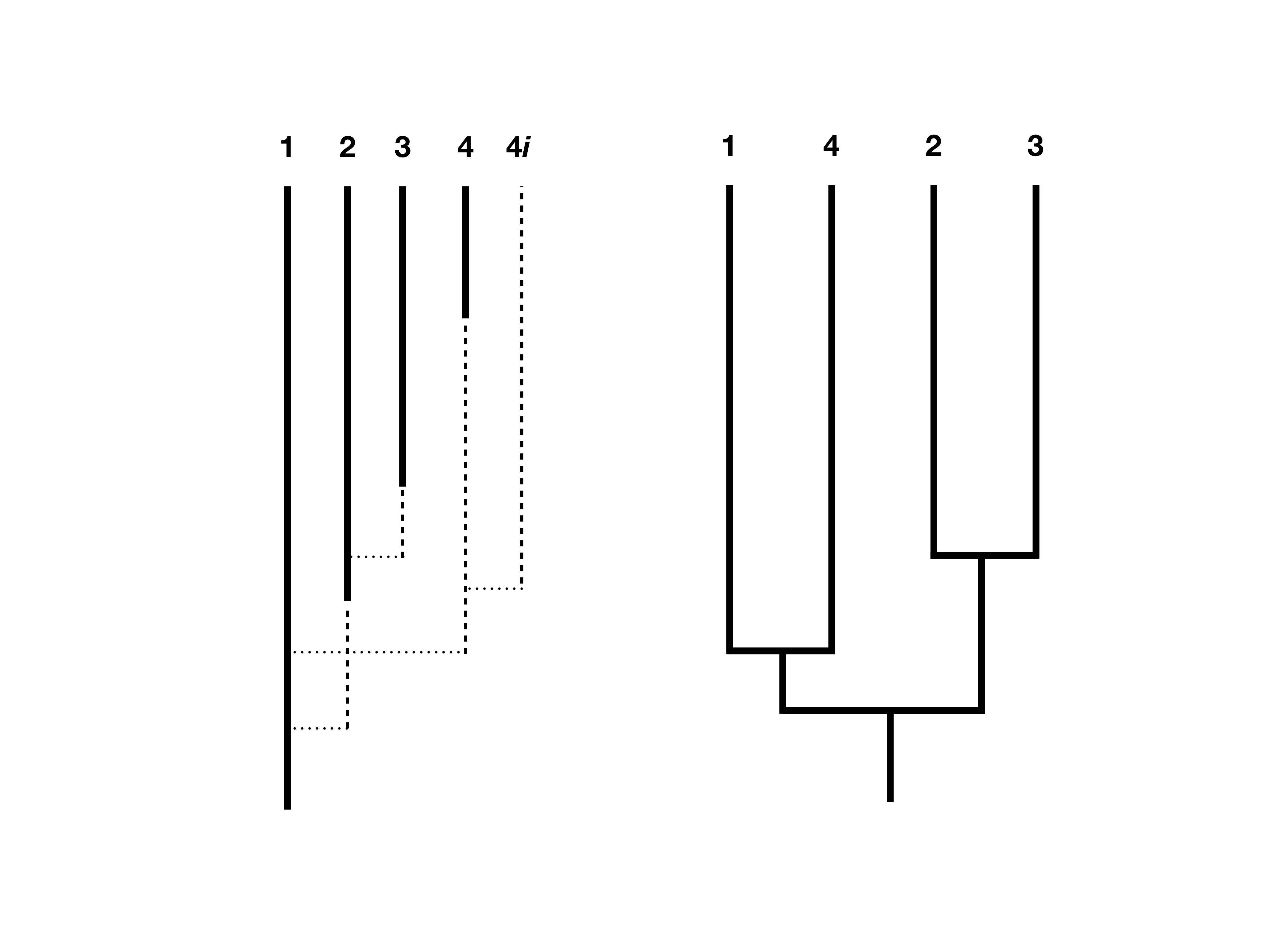
Figure 12.5. An illustration of the protracted model of speciation on a phylogenetic tree. Panel A shows the growing tree including full (solid lines) and incipient species (dotted lines). Incipient species become full at some rate, and if that does not occur before sampling then they are not included in the final species tree (panel B; e.g. lineage 4i). Redrawn from Lambert et al. (2015). Image by the author, can be reused under a CC-BY-4.0 license.
Because speciation takes time, the main impact of this model is that we predict fewer very young species in our tree – that is, the nodes closest to the tips of the tree are not as young as they would be compared to pure-birth or birth-death models without protracted speciation (Figure 12.6). As a result, protracted speciation models produce lineage through time plots that can mimic the properties often attributed to diversity-dependence, even without any interactions among lineages (Etienne and Rosindell 2012)!
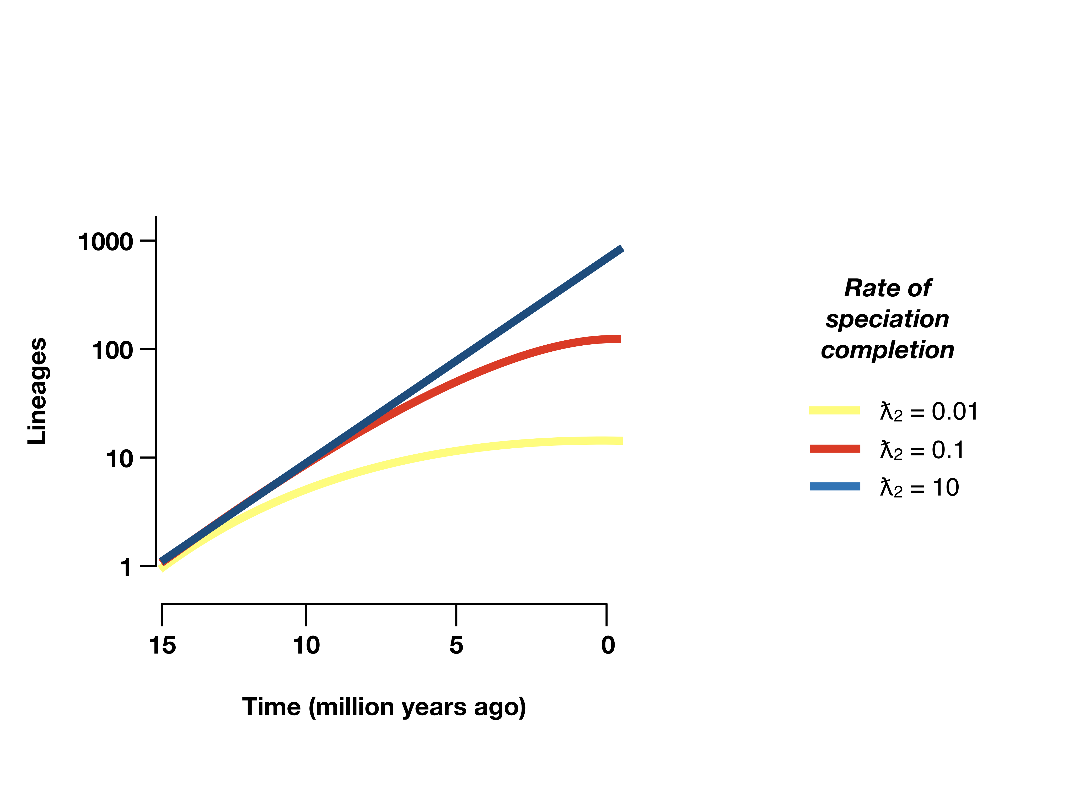
Figure 12.6. Lineage-through-time plots under a protracted birth-death model. Redrawn from Etienne and Rosindell (2012). Image by the author, can be reused under a CC-BY-4.0 license.
Likelihood approaches are available for this model of protracted speciation. Again, the likelihood must be calculated using numerical methods (Lambert et al. 2015). Fitting this model to the salamander tree, we obtain a maximum log-likeihood of 513.8 with parameter values λ1 = 0.059, λ2 = 0.44, and μ = 0.0. This corresponds to an AIC score of -1021.6; this model fits about as well as the best of the time-varying models but not as well as the diversity dependent model considered above. Again, though, I am not including plausible combinations of models, such as protracted speciation that varies through time.
So far, models of protracted speciation remain mostly in the realm of ecological neutral theory, and are just beginning to move into phylogenetics and evolutionary biology (see, e.g., Sukumaran and Lacey Knowles 2017). However, I think models that treat speciation as a process that takes time – rather than something instantaneous – will be an important addition to our macroevolutionary toolbox in the future.
Section 12.5: Summary
In this chapter I discussed models that go beyond constant rate birth-death models. We can fit models where speciation rate varies across clades or through time (or both). In some cases, very different models predict the same pattern in phylogenetic trees, warranting some caution until direct fossil data can be incorporated. I also described a model of protracted speciation, where speciation takes some time to complete. This latter model is potentially better connected to microevolutionary models of speciation, and could point towards fruitful directions for the field. We know that simple birth-death models do not capture the richness of speciation and extinction across the tree of life, so these models that range beyond birth and death are critical to the growth of comparative methods.
Footnotes
1: Even though this approach requires topology, Morlon et al. (2011) show that their likelihood is equivalent to other approaches, such as Nee and Maddison, that rely only on branching times and ignore topology completely. This is because trees with the same set of branching times but different topologies have identical likelihoods under this model.
References
Alfaro, M. E., F. Santini, C. Brock, H. Alamillo, A. Dornburg, D. L. Rabosky, G. Carnevale, and L. J. Harmon. 2009. Nine exceptional radiations plus high turnover explain species diversity in jawed vertebrates. Proceedings of the National Academy of Sciences 106:13410–13414. National Acad Sciences.
Benton, M. J. 2009. The red queen and the court jester: Species diversity and the role of biotic and abiotic factors through time. Science 323:728–732.
Brock, C. D., L. J. Harmon, and M. E. Alfaro. 2011. Testing for temporal variation in diversification rates when sampling is incomplete and nonrandom. Syst. Biol. 60:410–419. Oxford University Press.
Coyne, J. A., and H. A. Orr. 2004. Speciation. Sinauer, New York.
Cusimano, N., and S. S. Renner. 2010. Slowdowns in diversification rates from real phylogenies may not be real. Syst. Biol. 59:458–464.
De Queiroz, K. 2005. Ernst Mayr and the modern concept of species. Proceedings of the National Academy of Sciences 102:6600–6607. National Acad Sciences.
Emerson, B. C., and N. Kolm. 2005. Species diversity can drive speciation. Nature 434:1015–1017.
Etienne, R. S., and B. Haegeman. 2012. A conceptual and statistical framework for adaptive radiations with a key role for diversity dependence. Am. Nat. 180:E75–89.
Etienne, R. S., and J. Rosindell. 2012. Prolonging the past counteracts the pull of the present: Protracted speciation can explain observed slowdowns in diversification. Syst. Biol. 61:204–213.
Etienne, R. S., B. Haegeman, T. Stadler, T. Aze, P. N. Pearson, A. Purvis, and A. B. Phillimore. 2012. Diversity-dependence brings molecular phylogenies closer to agreement with the fossil record. Proc. Biol. Sci. 279:1300–1309.
Etienne, R. S., A. L. Pigot, and A. B. Phillimore. 2016. How reliably can we infer diversity-dependent diversification from phylogenies? Methods Ecol. Evol. 7:1092–1099.
Höhna, S. 2014. Likelihood inference of non-constant diversification rates with incomplete taxon sampling. PLoS One 9:e84184.
Hughes, C., and R. Eastwood. 2006. Island radiation on a continental scale: Exceptional rates of plant diversification after uplift of the Andes. Proc. Natl. Acad. Sci. U. S. A. 103:10334–10339.
Jetz, W., and R. A. Pyron. 2018. The interplay of past diversification and evolutionary isolation with present imperilment across the amphibian tree of life. Nat Ecol Evol 2:850–858.
Lambert, A., H. Morlon, and R. S. Etienne. 2015. The reconstructed tree in the lineage-based model of protracted speciation. J. Math. Biol. 70:367–397.
Losos, J. B., and F. R. Adler. 1995. Stumped by trees? A generalized null model for patterns of organismal diversity. Am. Nat. 145:329–342.
Losos, J. B., and D. Schluter. 2000. Analysis of an evolutionary species–area relationship. Nature 408:847. Macmillian Magazines Ltd.
May, M. R., and B. R. Moore. 2016. How well can we detect lineage-specific diversification-rate shifts? A simulation study of sequential AIC methods. Syst. Biol. 65:1076–1084.
Moen, D., and H. Morlon. 2014. Why does diversification slow down? Trends Ecol. Evol. 29:190–197.
Moore, B. R., S. Höhna, M. R. May, B. Rannala, and J. P. Huelsenbeck. 2016. Critically evaluating the theory and performance of Bayesian analysis of macroevolutionary mixtures. Proc. Natl. Acad. Sci. U. S. A. 113:9569–9574.
Morlon, H., T. L. Parsons, and J. B. Plotkin. 2011. Reconciling molecular phylogenies with the fossil record. Proc. Natl. Acad. Sci. U. S. A. 108:16327–16332. National Academy of Sciences.
Phillimore, A. B., and T. D. Price. 2008. Density-dependent cladogenesis in birds. PLoS Biol. 6:e71.
Pybus, O. G., and P. H. Harvey. 2000. Testing macro-evolutionary models using incomplete molecular phylogenies. Proc. Biol. Sci. 267:2267–2272.
Rabosky, D. L. 2014. Automatic detection of key innovations, rate shifts, anddiversity-dependence on phylogenetic trees. PLoS One 9:e89543. Public Library of Science.
Rabosky, D. L. 2013. Diversity-Dependence, ecological speciation, and the role of competition in macroevolution. Annu. Rev. Ecol. Evol. Syst. 44:481–502. annualreviews.org.
Rabosky, D. L. 2017. How to make any method “fail”: BAMM at the kangaroo court of false equivalency.
Rabosky, D. L., and A. H. Hurlbert. 2015. Species richness at continental scales is dominated by ecological limits. Am. Nat. 185:572–583.
Rabosky, D. L., and I. J. Lovette. 2008. Density-dependent diversification in North American wood warblers. Proc. Biol. Sci. 275:2363–2371.
Rabosky, D. L., S. C. Donnellan, A. L. Talaba, and I. J. Lovette. 2007. Exceptional among-lineage variation in diversification rates during the radiation of Australia’s most diverse vertebrate clade. Proc. Biol. Sci. 274:2915–2923.
Roelants, K., D. J. Gower, M. Wilkinson, and others. 2007. Global patterns of diversification in the history of modern amphibians. Proceedings of the. National Acad Sciences.
Rosindell, J., S. J. Cornell, S. P. Hubbell, and R. S. Etienne. 2010. Protracted speciation revitalizes the neutral theory of biodiversity. Ecol. Lett. 13:716–727.
Schluter, D. 2000. The ecology of adaptive radiation. Oxford University Press, Oxford.
Sepkoski, J. J. 1984. A kinetic model of phanerozoic taxonomic diversity. III. Post-Paleozoic families and mass extinctions. Paleobiology 10:246–267.
Slater, G. J., and L. J. Harmon. 2013. Unifying fossils and phylogenies for comparative analyses of diversification and trait evolution. Methods Ecol. Evol. 4:699–702. Wiley Online Library.
Sukumaran, J., and L. Lacey Knowles. 2017. Multispecies coalescent delimits structure, not species. Proc. Natl. Acad. Sci. U. S. A. 114:1607–1612. National Academy of Sciences.