Phylogenetic Comparative Methods learning from trees
- Chapter 11: Fitting birth-death models
- Section 11.1: Hotspots of diversity
- Section 11.2: Clade age and diversity
- Section 11.3: Tree Balance
- Section 11.3a: Sister clades and the balance of individual nodes
- Section 11.3b: Balance of whole phylogenetic trees
- Section 11.4: Fitting birth-death models to branching times
- Section 11.5: Sampling and birth-death models
- Section 11.6: Summary
Chapter 11: Fitting birth-death models
Section 11.1: Hotspots of diversity
The number of species on the Earth remains highly uncertain, but our best estimates are around 10 million (Mora et al. 2011). This is a mind-boggling number, and far more than have been described. As far as we know, all of those species are descended from a single common ancestor that lived some 4.2 billion years ago (Hedges and Kumar 2009). All of these species formed by the process of speciation, the process by which one species splits into two (or more) descendants (Coyne and Orr 2004).
Some parts of the tree of life have more species than others. This imbalance in diversity tells us that speciation is much more common in some lineages than others (Mooers and Heard 1997). Likewise, numerous studies have argued that certain habitats are "hotbeds" of speciation (e.g. Hutter et al. 2017; Miller and Wiens 2017). For example, the high Andes ecosystem called the Páramo - a peculiar landscape of alien-looking plants and spectacled bears - might harbor the highest speciation rates on the planet (Madriñán et al. 2013).
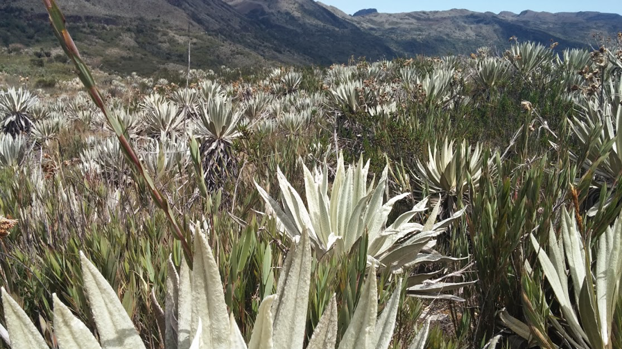
Figure 11.1 Páramo ecosystem, Chingaza Natural National Park, Colombia. Photo taken by the author, can be reused under a CC-BY-4.0 license.
In this chapter we will explore how we can learn about speciation and extinction rates from the tree of life. We will use birth-death models, simple models of how species form and go extinct through time. Birth-death models can be applied to data on clade ages and diversities, or fit to the branching times in phylogenetic trees. We will explore both maximum likelihood and Bayesian methods to do both of these things.
Section 11.2: Clade age and diversity
If we know the age of a clade and its current diversity, then we can calculate the net diversification rate for that clade. Before presenting equations, I want to make a distinction between two different ways that one can measure the age of a clade: the stem age and the crown age. A clade's crown age is the age of the common ancestor of all species in the clade. By contrast, a clade's stem age measures the time that that clade descended from a common ancestor with its sister clade. The stem age of a clade is always at least as old, and usually older, than the crown age.
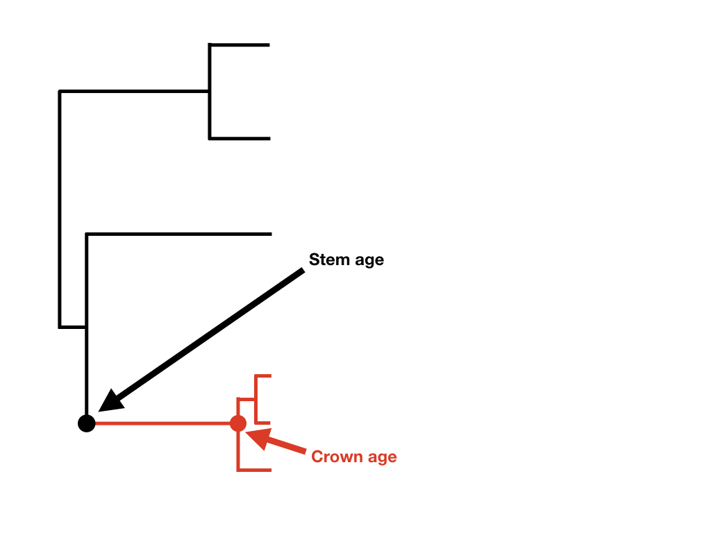
Figure 11.2. Crown and stem age of a clade of interest (highlighted in red). Image by the author, can be reused under a CC-BY-4.0 license.
Magallón and Sanderson (2001) give an equation for the estimate of net diversification rate given clade age and diversity:
(eq. 11.1)
$$
\hat{r} = \frac{ln(n)}{t_{stem}}
$$
where n is the number of species in the clade at the present day and tstem is the stem group age. In this equation we also see the net diversification rate parameter, r = λ − μ (see Chapter 10). This is a good reminder that this parameter best predicts how species accumulate through time and reflects the balance between speciation and extinction rates.
Alternatively, one can use tcrown, the crown group age:
(eq. 11.2)
$$
\hat{r} = \frac{ln(n)-ln(2)}{t_{crown}}
$$
The two equations differ because at the crown group age one is considering the clade's diversification starting with two lineages rather than one (Figure 11.2).
Even though these two equations reflect the balance of births and deaths through time, they give ML estimates for r only under a pure birth model where there is no extinction. If there has been extinction in the history of the clade, then our estimates using equations 11.1 and 11.2 will be biased. The bias comes from the fact that we see only clades that survive to the present day, and miss any clades of the same age that died out before they could be observed. By observing only the "winners" of the diversification lottery, we overestimate the net diversification rate. If we know the relative amount of extinction, then we can correct for this bias.
Under a scenario with extinction, one can define ϵ = μ/λ and use the following method-of-moments estimators from Rohatgi (1976, following the notation of Magallon and Sanderson (2001)):
(eq. 11.3)
$$
\hat{r} = \frac{log[n(1-\epsilon)+\epsilon]}{t_{stem}}
$$
for stem age, and
(eq. 11.4)
$$
\hat{r} = \frac{ln[\frac{n(1-\epsilon^2 )}{2}+2 \epsilon+\frac{(1-\epsilon) \sqrt{n(n \epsilon^2-8\epsilon+2 n \epsilon+n)}}{2}]-ln(2)}{t_{crown}}
$$
for crown age. (Note that eq. 11.3 and 11.4 reduce to 11.1 and 11.2, respectively, when ϵ = 0). Of course, we usually have little idea what ϵ should be. Common practice in the literature is to try a few different values for ϵ and see how the results change (e.g. Magallon and Sanderson 2001).
Magallón and Sanderson (2001), following Strathmann and Slatkin (1983), also describe how to use eq. 10.13 and 10.15 to calculate confidence intervals for the number of species at a given time.
As a worked example, let's consider the data in table 11.1, which give the crown ages and diversities of a number of plant lineages in the Páramo (from Madriñán et al. 2013). For each lineage, I have calculated the pure-birth estimate of speciation rate (from equation 11.2, since these are crown ages), and net diversification rates under three scenarios for extinction (ϵ = 0.1, ϵ = 0.5, and ϵ = 0.9).
| Lineage | n | Age | $\hat{r}_{pb}$ | $\hat{r}_{\epsilon = 0.1}$ | $\hat{r}_{\epsilon = 0.5}$ | $\hat{r}_{\epsilon = 0.9}$ |
|---|---|---|---|---|---|---|
| 1 | 17 | 0.42 | 5.10 | 5.08 | 4.53 | 2.15 |
| 2 | 14 | 10.96 | 0.18 | 0.18 | 0.16 | 0.07 |
| 3 | 32 | 3.80 | 0.73 | 0.73 | 0.66 | 0.36 |
| 4 | 65 | 2.50 | 1.39 | 1.39 | 1.28 | 0.78 |
| 5 | 55 | 3.05 | 1.09 | 1.08 | 1.00 | 0.59 |
| 6 | 120 | 4.04 | 1.01 | 1.01 | 0.94 | 0.62 |
| 7 | 36 | 4.28 | 0.68 | 0.67 | 0.61 | 0.34 |
| 8 | 32 | 7.60 | 0.36 | 0.36 | 0.33 | 0.18 |
| 9 | 66 | 1.47 | 2.38 | 2.37 | 2.19 | 1.34 |
| 10 | 27 | 8.96 | 0.29 | 0.29 | 0.26 | 0.14 |
| 11 | 5 | 3.01 | 0.30 | 0.30 | 0.26 | 0.09 |
| 12 | 46 | 0.80 | 3.92 | 3.91 | 3.58 | 2.07 |
| 13 | 53 | 14.58 | 0.22 | 0.22 | 0.21 | 0.12 |
The table above shows estimates of net diversification rates for Páramo lineages (data from Madriñán et al. 2013) using equations 11.2 and 11.4. Lineages are as follows: 1: Aragoa, 2: Arcytophyllum, 3: Berberis, 4: Calceolaria, 5: Draba, 6: Espeletiinae, 7: Festuca, 8: Jamesonia + Eriosorus, 9: Lupinus, 10: Lysipomia, 11: Oreobolus, 12: Puya, 13: Valeriana.
Inspecting the last four columns of this table, we can make a few general observations. First, these plant lineages really do have remarkably high diversification rates (Madriñán et al. 2013). Second, the net diversification rate we estimate depends on what we assume about relative extinction rates (ϵ). You can see in the table that the effect of extinction is relatively mild until extinction rates are assumed to be quite high (ϵ = 0.9). Finally, assuming different levels of extinction affects the diversification rates but not their relative ordering. In all cases, net diversification rates for Aragoa, which formed 17 species in less than half a million years, is higher than the rest of the clades. This relationship holds only when we assume relative extinction rates are constant across clades, though. For example, the net diversification rate we calculate for Calceolaria with ϵ = 0 is higher than the calculated rate for Aragoa with ϵ = 0.9. In other words, we can't completely ignore the role of extinction in altering our view of present-day diversity patterns.
We can also estimate birth and death rates for clade ages and diversities using ML or Bayesian approaches. We already know the full probability distribution for birth-death models starting from any standing diversity N(0)=n0 (see equations 10.13 and 10.15). We can use these equations to calculate the likelihood of any particular combination of N and t (either tstem or tcrown) given particular values of λ and μ. We can then find parameter values that maximize that likelihood. Of course, with data from only a single clade, we cannot estimate parameters reliably; in fact, we are trying to estimate two parameters from a single data point, which is a futile endeavor. (It is common, in this case, to assume some level of extinction and calculate net diversification rates based on that, as we did in Table 11.1 above).
One can also assume that a set of clades have the same speciation and extinction rates and fit them simultaneously, estimating ML parameter values. This is the approach taken by Magallón and Sanderson (2001) in calculating diversification rates across angiosperms. When we apply this approach to the Paramo data, shown above, we obtain ML estimates of $\hat{r} = 0.27$ and $\hat{\epsilon} = 0$. If we were forced to estimate an overall average rate of speciation for all of these clades, this might be a reasonable estimate. However, the table above also suggests that some of these clades are diversifiying faster than others. We will return to the issue of variation in diversification rates across clades in the next chapter.
We can also use a Bayesian approach to calculate posterior distributions for birth and death rates based on clade ages and diversities. This approach has not, to my knowledge, been implemented in any software package, although the method is straightforward (for a related approach, see Höhna et al. 2016). To do this, we will modify the basic algorithm for Bayesian MCMC (see Chapter 2) as follows:
Sample a set of starting parameter values, r and ϵ, from their prior distributions. For this example, we can set our prior distribution for both parameters as exponential with a mean and variance of λprior (note that your choice for this parameter should depend on the units you are using, especially for r). We then select starting r and ϵ from their priors.
Given the current parameter values, select new proposed parameter values using the proposal density Q(p′|p). For both parameter values, we can use a uniform proposal density with width wp, so that Q(p′|p) U(p − wp/2, p + wp/2). We can either choose both parameter values simultaneously, or one at a time (the latter is typically more effective).
Calculate three ratios:
- a. The prior odds ratio. This is the ratio of the probability of drawing the parameter values p and p′ from the prior. Since we have exponential priors for both parameters, we can calculate this ratio as (eq. 11.5):
$$ R_{prior} = \frac{\lambda_{prior} e^{-\lambda_{prior} p'}}{\lambda_{prior} e^{-\lambda_{prior} p}}=e^{\lambda_{prior} (p-p')} $$
- a. The prior odds ratio. This is the ratio of the probability of drawing the parameter values p and p′ from the prior. Since we have exponential priors for both parameters, we can calculate this ratio as (eq. 11.5):
- b. The proposal density ratio. This is the ratio of probability of proposals going from p to p′ and the reverse. We have already declared a symmetrical proposal density, so that Q(p′|p)=Q(p|p′) and Rproposal = 1.
- c. The likelihood ratio. This is the ratio of probabilities of the data given the two different parameter values. We can calculate these probabilities from equations 10.13 or 10.16 (depending on if the data are stem ages or crown ages).
- Find Raccept as the product of the prior odds, proposal density ratio, and the likelihood ratio. In this case, the proposal density ratio is 1, so (eq. 11.6):
Raccept = Rprior ⋅ Rlikelihood - Draw a random number u from a uniform distribution between 0 and 1. If u < Raccept, accept the proposed value of both parameters; otherwise reject, and retain the current value of the two parameters.
- Repeat steps 2-5 a large number of times.
When we apply this technique to the Páramo (from Madriñán et al. 2013) and priors with λprior = 1 for both r and ϵ, we obtain posterior distributions: r (mean = 0.497, 95% CI = 0.08-1.77) and ϵ (mean = 0.36, 95% CI = 0.02-0.84; Figure 11.3). Note that these results are substantially different than the ML estimates. This could be because in our Bayesian analysis our prior on extinction rates is exponential, and taking the posterior mean gives a high probability for relatively strong levels of extinction relative to speciation.
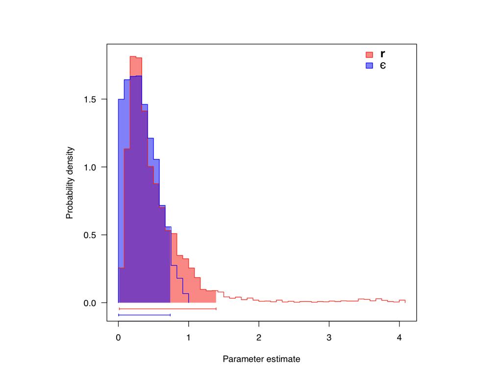
Figure 11.3. Posterior distribution for r and ϵ for Páramo clades. Data from Madriñán et al. (2013), image by the author, can be reused under a CC-BY-4.0 license.
Thus, we can estimate diversification rates from data on clade ages and diversities. If we have a whole set of such clades, we can (in principal) estimate both speciation and extinction rates, so long as we are willing to assume that all of the clades share equal diversification rates. However, as we will see in the next section, this assumption is almost always dubious!
Section 11.3: Tree Balance
As we discussed in Chapter 10, tree balance considers how "balanced" the branches of a phylogenetic tree are. That is, if we look at each node in the tree, are the two sister clades of the same size (balanced) or wildly different (imbalanced)?
Birth-death trees have a certain amount of "balance," perhaps a bit less than your intuition might suggest (see chapter 10). We can look to real trees to see if the amount of balance matches what we expect under birth-death models. A less balanced pattern in real trees would suggest that speciation and/or extinction rate vary among lineages more than we would expect. By contrast, more balanced trees would suggest more even and predictable diversification across the tree of life than expected under birth-death models. This approach traces back to Raup and colleagues, who applied stochastic birth-death models to paleontology in a series of influential papers in the 1970s (e.g. Raup et al. 1973, Raup and Gould (1974)). I will show how to do this for both individual nodes and for whole trees in the following sections.
Section 11.3a: Sister clades and the balance of individual nodes
For single nodes, we already know that the distribution of sister taxa species richness is uniform over all possible divisions of Nn species into two clades of size Na and Nb (Chapter 11). This idea leads to simple test of whether the distribution of species between two sister clades is unusual compared to the expectation under a birth-death model (Slowinski and Guyer 1993). This test can be used, for example, to test whether the diversity of exceptional clades, like passerine birds, is higher than one would expect when compared to their sister clade. This is the simplest measure of tree balance, as it only considers one node in the tree at a time.
Slowinsky and Guyer (1993) developed a test based on calculating a P-value for a division at least as extreme as seen in a particular comparison of sister clades. We consider Nn total species divided into two sister clades of sizes Na and Nb, where Na < Nb and Na + Nb = Nn. Then:
(eq. 11.7) If Na ≠ Nb:
$$
P = \frac{2 N_a}{N_n - 1}
$$
If Na = Nb or P > 1 then set P = 1
For example, we can assess diversification in the Andean representatives of the legume genus Lupinus (Hughes and Eastwood 2006). This genus includes one young radiation of 81 Andean species, spanning a wide range of growth forms. The likely sister clade to this spectacular Andean radiation is a clade of Lupinus species in Mexico that includes 46 species (Drummond et al. 2012). In this case Na = 81 − 46 = 35, and we can then calculate a P-value testing the null hypothesis that both of these clades have the same diversification rate:
(eq. 11.8)
$$
P = \frac{2 N_a}{N_n - 1} = \frac{2 \cdot 35}{81 - 1} = 0.875
$$
We cannot reject the null hypothesis. Indeed, later work suggests that the actual increase in diversification rate for Lupinus occurred deeper in the phylogenetic tree, in the ancestor of a more broadly ranging New World clade (Hughes and Eastwood 2006; Drummond et al. 2012).
Often, we are interested in testing whether a particular trait - say, dispersal into the Páramo - is responsible for the increase in species richness that we see in some clades. In that case, a single comparison of sister clades may be unsatisfying, as sister clades almost always differ in many characters, beyond just the trait of interest. Even if the clade with our putative "key innovation" is more diverse, we still might not be confident in inferring a correlation from a single observation. We need replication.
To address this problem, many studies have used natural replicates across the tree of life, comparing the species richnesses of many pairs of sister clades that differ in a given trait of interest. Following Slowinsky and Guyer (1993), we could calculate a p-value for each clade, and then combine those p-values into an overall test. In this case, one clade (with diversity N1) has the trait of interest and the other does not (N0), and our formula is half of equation 11.5 since we will consider this a one-tailed test:
(eq. 11.9)
$$
P = \frac{N_0}{N_n - 1}
$$
When analyzing replicate clade comparisons - e.g. many sister clades, where in each case one has the trait of interest and the other does not - Slowinsky and Guyer (1993) recommended combining these p-values using Fisher's combined probability test, so that:
(eq. 11.10)
χ2combined = −2∑ln(Pi)
Here, the Pi values are from i independent sister clade comparisons, each using equation 11.9. Under the null hypothesis where the character of interest does not increase diversification rates, the test statistic, χ2combined, should follow a chi-squared distribution with 2k degrees of freedom where k is the number of tests. But before you use this combined probability approach, see what happens when we apply it to a real example!
As an example, consider the following data, which compares the diversity of many sister pairs of plants. In each case, one clade has fleshy fruits and the other dry (data from Vamosi and Vamosi 2005):
| Fleshy fruit clade | nfleshy | Dry fruit clade | ndry |
|---|---|---|---|
| A | 1 | B | 2 |
| C | 1 | D | 64 |
| E | 1 | F | 300 |
| G | 1 | H | 89 |
| I | 1 | J | 67 |
| K | 3 | L | 4 |
| M | 3 | N | 34 |
| O | 5 | P | 10 |
| Q | 9 | R | 150 |
| S | 16 | T | 35 |
| U | 33 | V | 2 |
| W | 40 | X | 60 |
| Y | 50 | Z | 81 |
| AA | 100 | BB | 1 |
| CC | 216 | DD | 3 |
| EE | 393 | FF | 1 |
| GG | 850 | HH | 11 |
| II | 947 | JJ | 1 |
| KK | 1700 | LL | 18 |
The clades in the above table are as follows: A: Pangium, B: Acharia+Kigellaria, C: Cyrilla, D: Clethra, E: Roussea, F: Lobelia, G: Myriophylum + Haloragis + Penthorum, H: Tetracarpaea, I: Austrobaileya, J: Illicium+Schisandra, K: Davidsonia, L: Bauera, M: Mitchella, N: Pentas, O: Milligania , P: Borya, Q: Sambucus, R: Viburnum, S: Pereskia, T: Mollugo, U: Decaisnea + Sargentodoxa + Tinospora + Menispermum + Nandina Caulophyllum + Hydrastis + Glaucidium, V: Euptelea, W: Tetracera, X: Dillenia, Y: Osbeckia, Z: Mouriri, AA: Hippocratea, BB: Plagiopteron, CC: Cyclanthus + Sphaeradenia + Freycinetia, DD: Petrosavia + Japonlirion, EE: Bixa, FF: Theobroma + Grewia + Tilia + Sterculia + Durio, GG: Impatiens, HH: Idria, II: Lamium + Clerodendrum + Callicarpa + Phyla + Pedicularis + Paulownia, JJ: Euthystachys, KK: Callicarpa + Phyla + Pedicularis + Paulownia + Solanum, LL: Solanum.
The individual clades show mixed support for the hypothesis, with only 7 of the 18 comparisons showing higher diversity in the fleshy clade, but 6 of those 7 comparisons significant at P < 0.05 using equation 11.9. The combined probability test gives a test statistic of χ2combined = 72.8. Comparing this to a χ2 distribution with 36 degrees of freedom, we obtain P = 0.00027, a highly significant result. This implies that fleshy fruits do, in fact, result in a higher diversification rate.
However, if we test the opposite hypothesis, we see a problem with the combined probability test of equation 11.10 (Vamosi and Vamosi 2005). First, notice that 11 of 18 comparisons show higher diversity in the non-fleshy clade, with 4 significant at P < 0.05. The combined probability test gives χ2combined = 58.9 and P = 0.0094. So we reject the null hypothesis and conclude that non-fleshy fruits diversify at a higher rate! In other words, we can reject the null hypothesis in both directions with this example.
What's going on here? It turns out that this test is very sensitive to outliers - that is, clades with extreme differences in diversity. These clades are very different than what one would expect under the null hypothesis, leading to rejection of the null - and, in some cases with two characters, when there are outliers on both sides (e.g. the proportion of species in each state has a u-shaped distribution; Paradis 2012) we can show that both characters significantly increase diversity (Vamosi and Vamosi 2005)!
Fortunately, there are a number of improved methods that can be used that are similar in spirit to the original Slowinsky and Guyer test but more statistically robust (e.g Paradis 2012). For example, we can apply the "richness Yule test" as described in Paradis (2012), to the data from Vamosi et al. (2005). This is a modified version of the McConway-Sims test (McConway and Sims 2004), and compares the likelihood of a equal rate yule model applied to all clades to a model where one trait is associated with higher or lower diversification rates. This test requires knowledge of clade ages, which I don't have for these data, but Paradis (2012) shows that the test is robust to this assumption and recommends substituting a large and equal age for each clade. I chose 1000 as an arbitrary age, and found a significant likelihood ratio test (null model lnL = −215.6, alternative model lnL = −205.7, P = 0.000008). This method estimates a higher rate of diversification for fleshy fruits (since the age of the clade is arbitrary, the actual rates are not meaningful, but their estimated ratio λ1/λ0 = 1.39 suggests that fleshy fruited lineages have a diversification rate almost 40% higher).
Section 11.3b: Balance of whole phylogenetic trees
We can assess the overall balance of an entire phylogenetic tree using tree balance statistics. As discussed, I will describe just one common statistic, Colless' I, since other metrics capture the same pattern in slightly different ways.
To calculate Colless' I, we can use equation 10.18. This result will depend strongly on tree size, and so is not comparable across trees of different sizes; to allow comparisons, Ic is usually standardized by subtracting the expected mean for trees of that size under an random model (see below), and dividing by the standard deviation. Both of these can be calculated analytically (Blum et al. 2006), and standardized Ic calculated using a small approximation (following Bortolussi et al. 2006) as:
(eq. 11.11)
$$
I^{'}_c = \frac{I_c-n*log(n)-n(\gamma-1-log(2))}{n}
$$
Since the test statistics are based on descriptions of patterns in trees rather than particular processes, the relationship between imbalance and evolutionary processes can be difficult to untangle! But all tree balance indices allow one to reject the null hypothesis that the tree was generated under a birth-death model. Actually, the expected patterns of tree balance are absolutely identical under a broader class of models called "Equal-Rates Markov" (ERM) models (Harding 1971; Mooers and Heard 1997). ERM models specify that diversification rates (both speciation and extinction) are equal across all lineages for any particular point in time. However, those rates may or may not change through time. If they don't change through time, then we have a constant rate birth-death model, as described above - so birth-death models are ERM models. But ERM models also include, for example, models where birth rates slow through time, or extinction rates increase through time, and so on. As long as the changes in rates occur in exactly the same way across all lineages at any time, then all of these models predict exactly the same pattern of tree balance.
Typical steps for using tree balance indices to test the null hypothesis that the tree was generated under an ERM model are as follows:
- Calculate tree balance using a tree balance statistic.
- Simulate pure birth trees to general a null distribution of the test statistic. We are considering the set of ERM models as our null, but since pure-birth is simple and still ERM we can use it to get the correct null distribution.
- Compare the actual test statistic to the null distribution. If the actual test statistic is in the tails of the null distribution, then your data deviates from an ERM model.
Step 2 is unnecessary in cases where we know null distributions for tree balance statistics analytically, true for some (but not all) balance metrics (e.g. Blum and François 2006). There are also some examples in the literature of considering null distributions other than ERM. For example, Mooers and Heard (1997) consider two other null models, PDA and EPT, which consider different statistical distributions of tree shapes (but both of these are difficult to tie to any particular evolutionary process).
Typically, phylogenetic trees are more imbalanced than expected under the ERM model. In fact, this is one of the most robust generalizations that one can make about macroevolutionary patterns in phylogenetic trees. This deviation means that diversification rates vary among lineages in the tree of life. We will discuss how to quantify and describe this variation in later chapters. These tests are all similar in that they use multiple non-nested comparisons of species richness in sister clades to calculate a test statistic, which is then compared to a null distribution, usually based on a constant-rates birth-death process (reviewed in Vamosi and Vamosi 2005; Paradis 2012).
As an example, we can apply the whole-tree balance approach to the tree of Lupinus (Drummond et al. 2012). For this tree, which has 137 tips, we calculate Ic = 1010 and Ic′ = 3.57. This is much higher than expected by chance under an ERM model, with P = 0.0004. That is, our tree is significantly more imbalanced than expected under a ERM model, which includes both pure birth and birth-death. We can safely conclude that there is variation in speciation and/or extinction rates across lineages in the tree.
Section 11.4: Fitting birth-death models to branching times
Another approach that uses more of the information in a phylogenetic tree involves fitting birth-death models to the distribution of branching times. This approach traces all the way back to Yule (1925), who first applied stochastic process models to the growth of phylogenetic trees. More recently, a series of papers by Raup and colleagues (Raup et al. 1973; Raup and Gould 1974; Gould et al. 1977; Raup 1985) spurred modern approaches to quantitative macroevolution by simulating random clades, then demonstrating how variable such clades grown under simple birth-death models can be.
Most modern approaches to fitting birth-death models to phylogenetic trees use the intervals between speciation events on a tree - the "waiting times" between successive speciation - to estimate the parameters of birth-death models. Figure 10.2 shows these waiting times. Frequently, information about the pattern of species accumulation in a phylogenetic tree is summarized by a lineage-through-time (LTT) plot, which is a plot of the number of lineages in a tree against time (see Figure 10.9). As I introduced in Chapter 10, the y-axis of LTT plots is log-transformed, so that the expected pattern under a constant-rate pure-birth model is a straight line. Note also that LTT plots ignore the relative order of speciation events. Stadler (2013b) calls models justifying such an approach "species-exchangable" models - we can change the identity of species at any time point without changing the expected behavior of the model. Because of this, approaches to understanding birth-death models based on branching times are different from - and complementary to - approaches based on tree topology, like tree balance.
As discussed in the previous chapter, even though we often have no information about extinct species in a clade, we can still (in theory) infer the presence of extinction from an LTT plot. The signal of extinction is an excess of young lineages, which is seen as the "pull of the recent" in our LTT plots (Figure 10.10). In the next chapter, I will demonstrate how statistical approaches can capture this pattern in a more rigorous way.
Section 11.4a: Likelihood of waiting times under a birth-death model
In order to use ML and Bayesian methods for estimating the parameters of birth-death models from comparative data, we need to write down the likelihoods of the waiting times between speciation events in a tree. There is a little bit of variation in notation in the literature, so I will follow Stadler (2013b) and Maddison et al. (2007), among others, to maintain consistency. We will assume that the clade begins at time t1 with a pair of species. Most analyses follow this convention, and condition the process as starting at the time t1, representing the node at the root of the tree. This makes sense because we rarely have information on the stem age of our clade. We will also condition on both of these initial lineages surviving to the present day, as this is a requirement to obtain a tree with this crown age (e.g. Stadler 2013a equation 5).
Speciation and extinction events occur at various times, and the process ends at time 0 when the clade has n extant species - that is, we measure time backwards from the present day. Extinction will result in species that do not extend all the way to time 0. For now, we will assume that we only have data on extant species. We will refer to the phylogenetic tree that shows branching times leading to the extant species as the reconstructed tree (Nee et al. 1994). For a reconstructed tree with n species, there are n − 1 speciation times, which we will denote as t1, t2, t3, ..., tn − 1. The leaves of our ultrametric tree all terminate at time 0.
Note that in this notation, t1 > t2 > … > tn − 1 > 0, that is, our speciation times are measured backwards from the tips, and as we increase the index the times are constantly decreasing [this is an important notational difference between Stadler (2013a), used here, and Nee (1994 and others), the latter of which considers the time intervals between speciation events, e.g. t1 − t2 in our notation]. For now, we will assume complete sampling; that is, all n species alive at the present day are represented in the tree.
We will now derive a likelihood of of observing the set of speciation times t1, t2, ..., tn − 1 given the extant diversity of the clade, n, and our birth-death model parameters λ and μ. To do this, we will follow very closely an approach based on differential equations introduced by Maddison et al. (2007).
The general idea is that we will assign values to these probabilities at the tips of the tree, and then define a set of rules to update them as we flow back through the tree from the tips to the root. When we arrive at the root of the tree, we will have the probability of observing the actual tree given our model - that is, the likelihood. This is another pruning algorithm.
To begin with, we need to keep track of two probabilities: DN(t), the probability that a lineage at some time t in the past will evolve into the extant clade N as observed today; and E(t), the probability that a lineage at some time t will go completely extinct and leave no descendants at the present day. (Later, we will redefine E(t) so that it includes the possibility that the lineages has descendants but none have been sampled in our data). We then apply these probabilities to the tree using three main ideas (Figure 11.4)
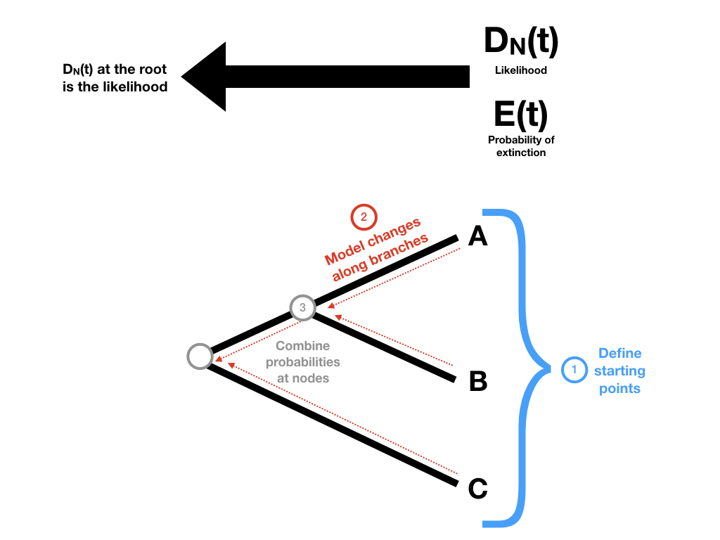
Figure 11.4. General outline of steps for calculating likelihood of a tree under a birth-death model. Image inspired by Maddison et al. (2007) and created by the author, can be reused under a CC-BY-4.0 license.
We define our starting points at the tips of the tree.
We define how the probabilities defined in (1) change as we move backwards along branches of the tree.
We define what happens to our probabilities at the tree nodes.
Then, starting at the tips of the tree, we make our way to the root. At each tip, we have a starting value for both DN(t) and E(t). We move backwards along the branches of the tree, updating both probabilities as we go using step 2. When two branches come togther at a node, we combine those probabilities using step 3.
In this way, we walk through the tree, starting with the tips and passing over every branch and node (Figure 11.4). When we get to the root we will have DN(troot), which is the full likelihood that we want.
You might wonder why we need to calculate both DN(t) and E(t) if the likelihood is captured by DN(t) at the root. The reason is that the probability of observing a tree is dependent on these extinction probabilities calculated back through time. We need to keep track of E(t) to know about DN(t) and how it changes. You will see below that E(t) appears directly in our differential equations for DN(t).
First, the starting point. Since every tip i represents a living lineage, we know it is alive at the present day - so we can define DN(t)=1. We also know that it will not go extinct before being included in the tree, so E(t)=0. This gives our starting values for the two probabilities at each tip in the tree (Figure 11.5).
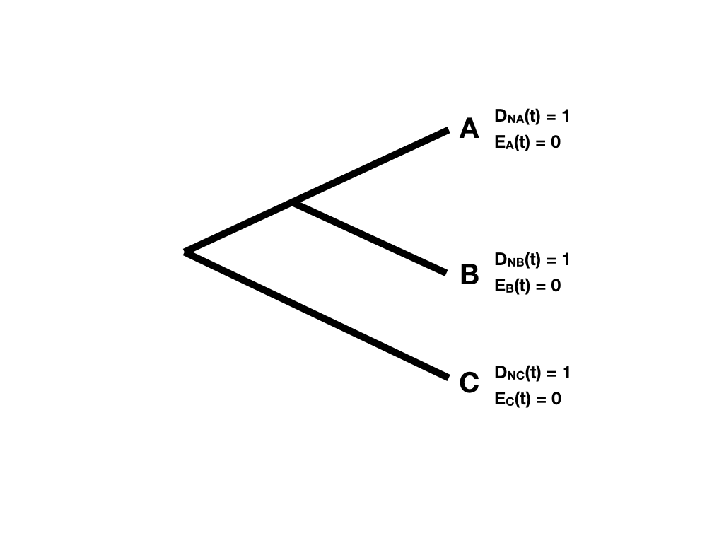
Figure 11.5. Starting points at tree tips for likelihood probability calculations. Image inspired by Maddison et al. (2007) and created by the author, can be reused under a CC-BY-4.0 license.
Next, imagine we move backwards along some section of a tree branch with no nodes. We will consider an arbitrary branch of the tree. Since we are going back in time, we will start at some node in the tree N, which occurs at a time tN, and denote the time going back into the past as t (Figure 11.6).
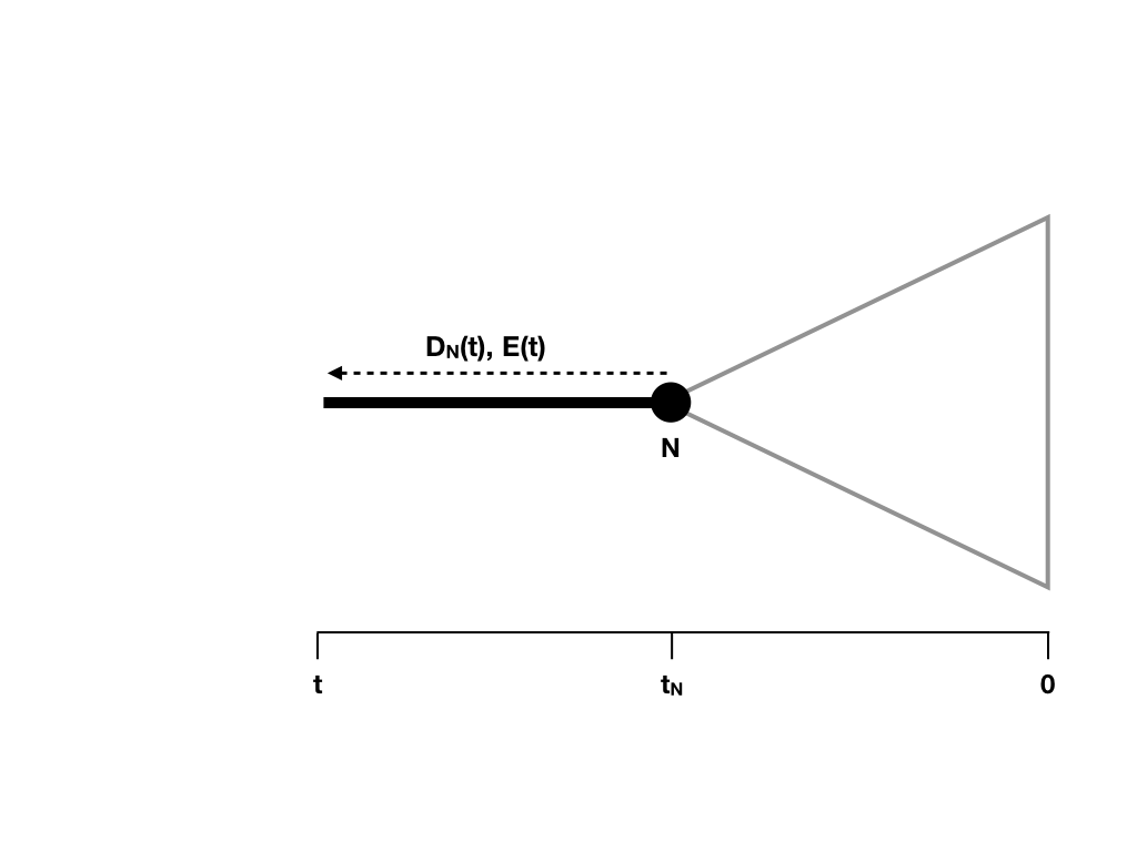
Figure 11.6. Updating DN(t) and calculating E(t) along a tree branch. Image inspired by Maddison et al. (2007) and created by the author, can be reused under a CC-BY-4.0 license.
Since that section of branch exists in our tree, we know two things: the lineage did not go extinct during that time, and if speciation occurred, the lineage that split off did not survive to the present day. We can capture these two possibilities in a differential equation that considers how our overall likelihood changes over some very small unit of time (Maddison et al. 2007).
(eq. 11.12)
$$
\frac{dD_N(t)}{dt} = -(\lambda + \mu) D_N(t) + 2 \lambda E(t) D_N(t)
$$
Here, the first part of the equation, −(λ + μ)DN(t), represents the probability of not speciating nor going extinct, while the second part, 2λE(t)DN(t), represents the probability of speciation followed by the ultimate extinction of one of the two daughter lineages. The 2 in this equation appears because we must account for the fact that, following speciation from an ancestor to daughters A and B, we would see the same pattern no matter which of the two descendants survived to the present.
We also need to calculate our extinction probability going back through the tree (Maddison et al. 2007):
(eq. 11.13)
$$
\frac{dE(t)}{dt} = \mu - (\mu + \lambda) E(t) + \lambda E(t)^2
$$
The three parts of this equation represent the three ways a lineage might not make it to the present day: either it goes extinct during the interval being considered (μ), it survives that interval but goes extinct some time later (−(μ + λ)E(t)), or it speciates in the interval but both descendants go extinct before the present day (λE(t)2) (Maddison et al. 2007). Unlike the DN(t) term, this probability depends only on time and not the topological structure of the tree.
We will also specify that λ > μ; it is possible to relax that assumption, but it makes the solution more complicated.
We can solve these equations so that we will be able to update the probability moving backwards along any branch of the tree with length t. First, solving equation 11.13 and using our initial condition E(0) = 0:
(eq. 11.14)
$$
E(t) = 1 - \frac{\lambda-\mu}{\lambda - (\lambda-\mu)e^{(\lambda - \mu)t}}
$$
We can now substitute this expression for E(t) into eq. 11.12 and solve.
(eq. 11.15)
$$
D_N(t) = e^{-(\lambda - \mu)(t - t_N)} \frac{(\lambda - (\lambda-\mu)e^{(\lambda - \mu)t_N})^2}{(\lambda - (\lambda-\mu)e^{(\lambda - \mu)t})^2} \cdot D_N(t_N)
$$
Remember that tN is the depth (measured from the present day) of node N (Figure 11.6).
Finally, we need to consider what happens when two branches come together at a node. Since there is a node, we know there has been a speciation event. We multiply the probability calculations flowing down each branch by the probability of a speciation event [Maddison et al. (2007); Figure 11.7].
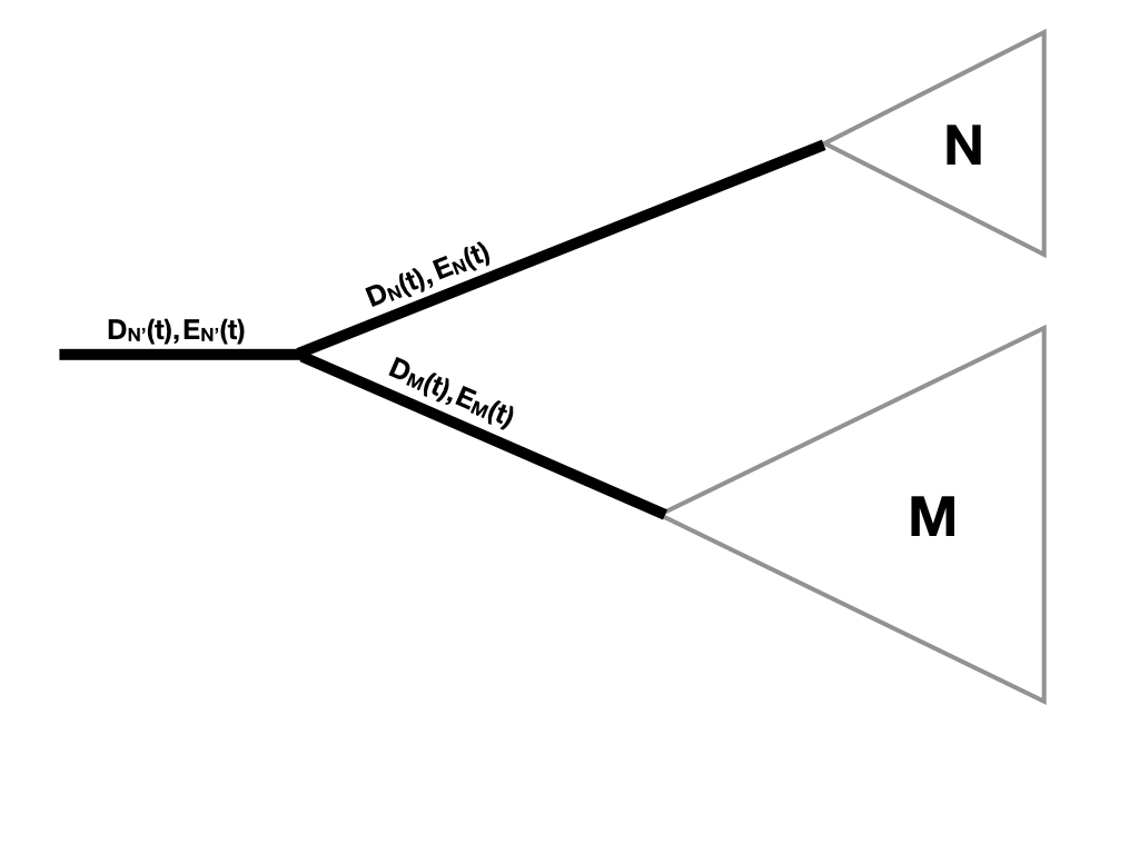
Figure 11.7. Updating DN(t) and E(t) along a tree branch. Image inspired by Maddison et al. (2007) and created by the author, can be reused under a CC-BY-4.0 license.
So:
(eq. 11.16)
DN′(t)=DN(t)DM(t)λ
Where clade N' is the clade made up of the combination of two sister clades N and M.
To apply this approach across an entire phylogenetic tree, we multiply equations 11.15 and 11.16 across all branches and nodes in the tree. Thus, the full likelihood is (Maddison et al. 2007; Morlon et al. 2011):
(eq. 11.17)
$$
L(t_1, t_2, \dots, t_n) = \lambda^{n-1} \big[ \prod_{k = 1}^{2n-2} e^{(\lambda-\mu)(t_{k,b} - t_{k,t})} \cdot \frac{(\lambda - (\lambda-\mu)e^{(\lambda - \mu)t_{k,t}})^2}{(\lambda - (\lambda-\mu)e^{(\lambda - \mu)t_{k,b}})^2} \big]
$$
Here, n is the number of tips in the tree (note that the original derivation in Maddison uses n as the number of nodes, but I have changed it for consistency with the rest of the book).
The product in equation 11.17 is taken over all 2n − 2 branches in the tree. Each branch k has two times associated with it, one towards the base of the tree, tk, b, and one towards the tips, tk, t.
Most methods fitting birth-death models to trees condition on the existence of a tree - that is, conditioning on the fact that the whole process did not go extinct before the present day, and the speciation event from the root node led to two surviving lineages. To do this conditioning, we divide equation 11.17 by λ[1 − E(troot)]2 (Morlon et al. 2011; Stadler 2013a).
Additionally, likelihoods for birth-death waiting times, for example those in the original derivation by Nee, include an additional term, (n − 1)!. This is because there are (n − 1)! possible topologies for any set of n − 1 waiting times, all equally likely. Since this term is constant for a given tree size n, then leaving it out has no influence on the relative likelihoods of different parameter values - but it is necessary to know about this multiplier if comparing likelihoods across different models for model selection, or comparing the output of different programs (Stadler 2013a).
Accounting for these two factors, the full likelihood is:
(eq. 11.18)
$$
L(\tau) = (n-1)! \frac{\lambda^{n-2} \big[ \prod_{k = 1}^{2n-2} e^{(\lambda-\mu)(t_{k,b} - t_{k,t})} \cdot \frac{(\lambda - (\lambda-\mu)e^{(\lambda - \mu)t_{k,t}})^2}{(\lambda - (\lambda-\mu)e^{(\lambda - \mu)t_{k,b}})^2} \big]}{ [1-E(t_{root})]^2}
$$
where:
(eq. 11.19)
$$
E(t_{root}) = 1 - \frac{\lambda-\mu}{\lambda - (\lambda-\mu)e^{(\lambda - \mu)t_{root}}}
$$
Section 11.4b: Using maximum likelihood to fit a birth-death model
Given equation 11.19 for the likelihood, we can estimate birth and death rates using both ML and Bayesian approaches. For the ML estimate, we maximize equation 11.19 over λ and μ. For a pure-birth model, we can set μ = 0, and the maximum likelihood estimate of λ can be calculated analytically as:
(eq. 11.20)
$$
\lambda= \frac{n-2}{s_{branch}}
$$
where sbranch is the sum of branch lengths in the tree,
(eq. 11.21)
$$
s_{branch} = \sum_{i=1}^{n-1} t_i + t_{n-1}
$$
Equation 11.21 is also called the Kendal-Moran estimator of the speciation rate (Nee 2006).
For a birth-death model, we can use numerical methods to maximize the likelihood over λ and μ.
For example, we can use ML to fit a birth-death model to the Lupinus tree (Drummond et al. 2012), which has 137 tip species and a total age of 16.6 million years. Doing so, we obtain ML parameter estimates of λ = 0.46 and μ = 0.20, with a log-likelihood of lnLbd = 262.3. Compare this to a pure birth model on the same tree, which gives λ = 0.35 and lnLpb = 260.4. One can compare the fit of these two models using AIC scores: AICbd = −520.6 and AICpb = −518.8, so the birth-death model has a better (lower) AIC score but by less than two AIC units. A likelihood ratio test, which gives Δ = 3.7 and P = 0.054. In other words, we estimate a non-zero extinction rate in the clade, but the evidence supporting that model over a pure-birth model is not particularly strong. Even if this model selection is a bit ambiguous, remember that we have also estimated parameters using all of the information that we have in the waiting times of the phylogenetic tree.
Section 11.4c: Using Bayesian MCMC to fit a birth-death model
We can also estimate birth and death rates using a Bayesian MCMC. We can use exactly the method spelled out above for clade ages and diversities, but substitute equation 11.11 for the likelihood, thus using the waiting times derived from a phylogenetic tree to estimate model parameters.
Applying this to Lupines with the same priors as before, we obtain the posterior distributions shown in figure 11.5. The mean of the posterior for each parameter is λ = 0.48 and μ = 0.23, quite close to the ML estimates for these parameters.
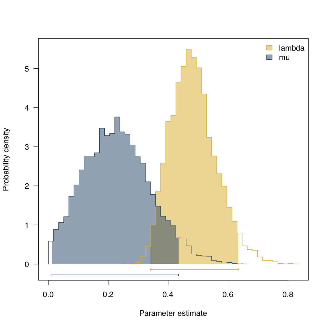
Figure 11.8. Posterior distribution for b and d for Lupinus. Data from (Drummond et al. 2012), image inspired by Maddison et al. (2007) and created by the author, can be reused under a CC-BY-4.0 license.
Section 11.5: Sampling and birth-death models
It is important to think about sampling when fitting birth-death models to phylogenetic trees. If any species are missing from your phylogenetic tree, they will lead to biased parameter estimates. This is because missing species are disproportionally likely to connect to the tree on short, rather than long, branches. If we randomly sample lineages from a tree, we will end up badly underestimating both speciation and extinction rates (and wrongly inferring slowdowns; see chapter 12).
Fortunately, the mathematics for incomplete sampling of reconstructed phylogenetic trees has also been worked out. There are two ways to do this, depending on how the tree is actually sampled. If we consider the missing species to be random with respect to the taxa included in the tree, then one can use a uniform sampling fraction to account for them. By contrast, we often are in the situation where we have tips in our tree that are single representatives of diverse clades (e.g. genera). We usually know the diversity of these unsampled clades in our tree of representatives. I will follow (Höhna et al. 2011; Höhna 2014) and refer to this approach as representative sampling (and the previous alternative as uniform sampling).
For the uniform sampling approach, we use the framework above of calculating backwards through time, but modify the starting points for each tip in the tree to reflect f, the probability of sampling a species (following Fitzjohn et al. (2009)):
(eq. 11.22)
DN(0)=1 − f
E(0)=f
Repeating the calculations above along branches and at nodes, but with the starting conditions above, we obtain the following likelihood (FitzJohn et al. 2009):
(eq. 11.23)
$$
\begin{aligned}
L(t_1, t_2, \dots, t_n) = \lambda^{n-1} \big[ \prod_{k = 1}^{2n-2} e^{(\lambda-\mu)(t_{k,b} - t_{k,t})} \cdot \\
\frac{(f \lambda - (\mu - \lambda(1-f))e^{(\lambda - \mu)t_{k,t}})^2}{(f \lambda - (\mu - \lambda(1-f))e^{(\lambda - \mu)t_{k,b}})^2} \big]
\end{aligned}
$$
Again, the above formula is proportional to the full likelihood, which is:
(eq. 11.24)
$$
L(\tau) = (n-1)! \frac{\lambda^{n-2} \big[ \prod_{k = 1}^{2n-2} e^{(\lambda-\mu)(t_{k,b} - t_{k,t})} \cdot \frac{(f \lambda - (\mu - \lambda(1-f))e^{(\lambda - \mu)t_{k,t}})^2}{(f \lambda - (\mu - \lambda(1-f))e^{(\lambda - \mu)t_{k,b}})^2} \big]}{[1-E(t_{root})]^2}
$$
and:
(eq. 11.25)
$$
E(t_{root}) = 1 - \frac{\lambda-\mu}{\lambda - (\lambda-\mu)e^{(\lambda - \mu)t_{root}}}
$$
For representative sampling, one approach is to consider the data as divided into two parts, phylogenetic and taxonomic. The taxonomic part is the stem age and extant diversity of the unsampled clades, while the phylogenetic part is the relationships among those clades. Following Rabosky and Lovette (2007), we can then calculate:
(eq. 11.26)
Ltotal = Lphylogenetic ⋅ Ltaxonomic
Where Lphylogenetic can be calculated using equation 11.18 and Ltaxonomic calculated for each clade using equation 10.16 and then multiplied to get the overall likelihood.
There are two extensions to this approach that are worth mentioning. One is Hohna's (2011) diversified sampling ("DS") model. This model makes a different assumption: when sampling n taxa from an overall set of m, the deepest n − 1 nodes have been included. Hohna's approach allows users to fit a model with representative sampling but without requiring assignment of extant diversity to each clade. Another approach, by Stadler and Smrckova (2016), calculates likelihoods for representatively sampled trees and can fit models of time-varying speciation and extinction rates (see chapter 12).
Section 11.6: Summary
In this chapter, I described how to estimate parameters from birth-death models using data on species diversity and ages, and how to use patterns of tree balance to test hypotheses about changing birth and death rates. I also described how to calculate the likelihood for birth-death models on trees, which leads directly to both ML and Bayesian methods for estimating birth and death rates. In the next chapter, we will explore elaborations on birth-death models, and discuss models that go beyond constant-rates birth-death models to analyze the diversity of life on Earth.
References
Blum, M. G. B., and O. François. 2006. Which random processes describe the tree of life? A large-scale study of phylogenetic tree imbalance. Syst. Biol. 55:685–691.
Blum, M. G. B., O. François, and S. Janson. 2006. The mean, variance and limiting distribution of two statistics sensitive to phylogenetic tree balance. Ann. Appl. Probab. 16:2195–2214. Institute of Mathematical Statistics.
Bortolussi, N., E. Durand, M. Blum, and O. François. 2006. ApTreeshape: Statistical analysis of phylogenetic tree shape. Bioinformatics 22:363–364.
Coyne, J. A., and H. A. Orr. 2004. Speciation. Sinauer, New York.
Drummond, C. S., R. J. Eastwood, S. T. S. Miotto, and C. E. Hughes. 2012. Multiple continental radiations and correlates of diversification in Lupinus (Leguminosae): Testing for key innovation with incomplete taxon sampling. Syst. Biol. 61:443–460. academic.oup.com.
FitzJohn, R. G., W. P. Maddison, and S. P. Otto. 2009. Estimating trait-dependent speciation and extinction rates from incompletely resolved phylogenies. Syst. Biol. 58:595–611. sysbio.oxfordjournals.org.
Gould, S. J., D. M. Raup, J. J. Sepkoski, T. J. M. Schopf, and D. S. Simberloff. 1977. The shape of evolution: A comparison of real and random clades. Paleobiology 3:23–40. Cambridge University Press.
Harding, E. F. 1971. The probabilities of rooted tree-shapes generated by random bifurcation. Adv. Appl. Probab. 3:44–77. Cambridge University Press.
Hedges, B. S., and S. Kumar. 2009. The timetree of life. Oxford University Press, Oxford.
Höhna, S. 2014. Likelihood inference of non-constant diversification rates with incomplete taxon sampling. PLoS One 9:e84184.
Höhna, S., M. R. May, and B. R. Moore. 2016. TESS: An R package for efficiently simulating phylogenetic trees and performing Bayesian inference of lineage diversification rates. Bioinformatics 32:789–791.
Höhna, S., T. Stadler, F. Ronquist, and T. Britton. 2011. Inferring speciation and extinction rates under different sampling schemes. Mol. Biol. Evol. 28:2577–2589.
Hughes, C., and R. Eastwood. 2006. Island radiation on a continental scale: Exceptional rates of plant diversification after uplift of the Andes. Proc. Natl. Acad. Sci. U. S. A. 103:10334–10339.
Hutter, C. R., S. M. Lambert, and J. J. Wiens. 2017. Rapid diversification and time explain amphibian richness at different scales in the tropical Andes, Earth’s most biodiverse hotspot. Am. Nat. 190:828–843.
Maddison, W. P., P. E. Midford, S. P. Otto, and T. Oakley. 2007. Estimating a binary character’s effect on speciation and extinction. Syst. Biol. 56:701–710. Oxford University Press.
Madriñán, S., A. J. Cortés, and J. E. Richardson. 2013. Páramo is the world’s fastest evolving and coolest biodiversity hotspot. Front. Genet. 4:192.
Magallon, S., and M. J. Sanderson. 2001. Absolute diversification rates in angiosperm clades. Evolution 55:1762–1780.
McConway, K. J., and H. J. Sims. 2004. A likelihood-based method for testing for nonstochastic variation of diversification rates in phylogenies. Evolution 58:12–23.
Miller, E. C., and J. J. Wiens. 2017. Extinction and time help drive the marine-terrestrial biodiversity gradient: Is the ocean a deathtrap? Ecol. Lett. 20:911–921.
Mooers, A. O., and S. B. Heard. 1997. Inferring evolutionary process from phylogenetic tree shape. Q. Rev. Biol. 72:31–54.
Mora, C., D. P. Tittensor, S. Adl, A. G. B. Simpson, and B. Worm. 2011. How many species are there on earth and in the ocean? PLoS Biol. 9:e1001127. Public Library of Science.
Morlon, H., T. L. Parsons, and J. B. Plotkin. 2011. Reconciling molecular phylogenies with the fossil record. Proc. Natl. Acad. Sci. U. S. A. 108:16327–16332. National Academy of Sciences.
Nee, S. 2006. Birth-Death models in macroevolution. Annu. Rev. Ecol. Evol. Syst. 37:1–17. Annual Reviews.
Nee, S., R. M. May, and P. H. Harvey. 1994. The reconstructed evolutionary process. Philos. Trans. R. Soc. Lond. B Biol. Sci. 344:305–311.
Paradis, E. 2012. Shift in diversification in sister-clade comparisons: A more powerful test. Evolution 66:288–295. Wiley Online Library.
Rabosky, D. L., S. C. Donnellan, A. L. Talaba, and I. J. Lovette. 2007. Exceptional among-lineage variation in diversification rates during the radiation of Australia’s most diverse vertebrate clade. Proc. Biol. Sci. 274:2915–2923.
Raup, D. M. 1985. Mathematical models of cladogenesis. Paleobiology 11:42–52.
Raup, D. M., and S. J. Gould. 1974. Stochastic simulation and evolution of morphology: Towards a nomothetic paleontology. Syst. Biol. 23:305–322. Oxford University Press.
Raup, D. M., S. J. Gould, T. J. M. Schopf, and D. S. Simberloff. 1973. Stochastic models of phylogeny and the evolution of diversity. J. Geol. 81:525–542.
Rohatgi, V. K. 1976. An introduction to probability theory and mathematical statistics. Wiley.
Slowinski, J. B., and C. Guyer. 1993. Testing whether certain traits have caused amplified diversification: An improved method based on a model of random speciation and extinction. Am. Nat. 142:1019–1024.
Stadler, T. 2013a. How can we improve accuracy of macroevolutionary rate estimates? Syst. Biol. 62:321–329.
Stadler, T. 2013b. Recovering speciation and extinction dynamics based on phylogenies. J. Evol. Biol. 26:1203–1219.
Stadler, T., and J. Smrckova. 2016. Estimating shifts in diversification rates based on higher-level phylogenies. Biol. Lett. 12:20160273. The Royal Society.
Strathmann, R. R., and M. Slatkin. 1983. The improbability of animal phyla with few species. Paleobiology. cambridge.org.
Vamosi, S. M., and J. C. Vamosi. 2005. Endless tests: Guidelines for analysing non-nested sister-group comparisons. Evol. Ecol. Res. 7:567–579. Evolutionary Ecology, Ltd.
Yule, G. U. 1925. A mathematical theory of evolution, based on the conclusions of dr. J. C. Willis, FRS. Philos. Trans. R. Soc. Lond. B Biol. Sci. 213:21–87. The Royal Society.