Phylogenetic Comparative Methods learning from trees
Chapter 5: Fitting Brownian Motion Models to Multiple Characters
Section 5.1: Introduction
As discussed in Chapter 4, body size is one of the most important traits of an animal. Body size has a close relationship to almost all of an animal’s ecological interactions, from whether it is a predator or prey to its metabolic rate. If that is true, we should be able to use body size to predict other traits that might be related through shared evolutionary processes. We need to understand how the evolution of body size is correlated with other species’ characteristics.
A wide variety of hypotheses can be framed as tests of correlations between continuously varying traits across species. For example, is the body size of a species related to its metabolic rate? How does the head length of a species relate to overall size, and do deviations from this relationship relate to an animal’s diet? These questions and others like them are of interest to evolutionary biologists because they allow us to test hypotheses about the factors in influencing character evolution over long time scales. These types of approaches allow us to answer some of the classic “why” questions in biology. Why are elephants so large? Why do some species of crocodilians have longer heads than others? If we find a correlation between two characters, we might suspect that there is a causal relationship between our two variables of interest - or perhaps that both of our measured variables share a common cause.
In this chapter, we will use the example of home range size, which is the area where an animal carries out its day-to-day activities. We will again use data from Garland (1992) and test for a relationship between body size and the size of a mammal’s home range. I will describe methods for using empirical data to estimate the parameters of multivariate Brownian motion models. I will then describe a model-fitting approach to test for evolutionary correlations. This model fitting approach is simple but not commonly used. Finally, I will review two common statistical approaches to test for evolutionary correlations, phylogenetic independent contrasts and phylogenetic generalized least squares, and describe their relationship to model-fitting approaches.
Section 5.2: What is evolutionary correlation?
There is sometimes a bit of confusion among beginners as to what, exactly, we are doing when we carry out a comparative method, especially when testing for character correlations. Common language that comparative methods “control for phylogeny” or “remove the phylogeny from the data” is not necessarily enlightening or even always accurate. Another common suggestion is that species are not statistically independent and that we must account for that with comparative methods. While accurate, I still don’t think this statement fully captures the tree-thinking perspective enabled by comparative methods. In this section, I will use the particular example of correlated evolution to try to illustrate the power of comparative methods and how they differ from standard statistical approaches that do not use phylogenies.
In statistics, two variables can be correlated with one another. We might refer to this as a standard correlation. When two traits are correlated, it means that given the value of one trait – say, body size in mammals – one can predict the value of another – like home range area. Correlations can be positive (large values of x are associated with large values of y) or negative (large values of x are associated with small values of y). A surprisingly wide variety of hypotheses in biology can be tested by evaluating correlations between characters.
In comparative biology, we are often interested more specifically in evolutionary correlations. Evolutionary correlations occur when two traits tend to evolve together due to processes like mutation, genetic drift, or natural selection. If there is an evolutionary correlation between two characters, it means that we can predict the magnitude and direction of changes in one character given knowledge of evolutionary changes in another. Just like standard correlations, evolutionary correlations can be positive (increases in trait x are associated with increases in y) or negative (decreases in x are associated with increases in y).
We can now contrast standard correlations, testing the relationships between trait values across a set of species, with evolutionary correlations - where evolutionary changes in two traits are related to each other. This is a key distinction, because phylogenetic relatedness alone can lead to a relationship between two variables that are not, in fact, evolving together (Figure 5.1; also see Felsenstein 1985). In such cases, standard correlations will, correctly, tell us that one can predict the value of trait y by knowing the value of trait x, at least among extant species; but we would be misled if we tried to make any evolutionary causal inference from this pattern. In the example of Figure 5.1, we can only predict x from y because the value of trait x tells us which clade the species belongs to, which, in turn, allows reasonable prediction of y. In fact, this is a classical example of a case where correlation is not causation: the two variables are only correlated with one another because both are related to phylogeny.
If we want to test hypotheses about trait evolution, we should specifically test evolutionary correlations1. If we find a relationship among the independent contrasts for two characters, for example, then we can infer that changes in each character are related to changes in the other – an inference that is much closer to most biological hypotheses about why characters might be related. In this case, then, we can think of statistical comparative methods as focused on disentangling patterns due to phylogenetic relatedness from patterns due to traits evolving in a correlated manner.
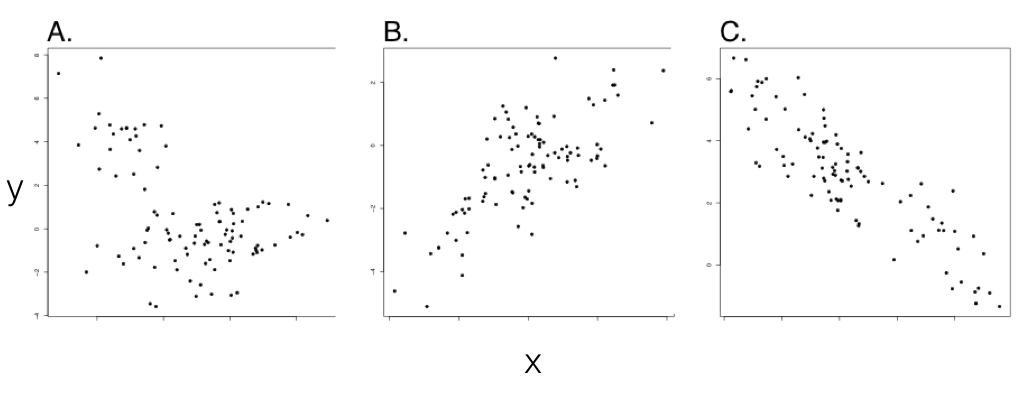
Figure 5.1. Examples from simulations of pure birth trees (b = 1) with n = 100 species. Plotted points represent character values for extant species in each clade. In all three panels, σx2 = σy2 = 1. σxy2 varies with σxy2 = 0 (panel A), σxy2 = 0.8 (panel B), and σxy2 = −0.8 (panel C). Note the (apparent) negative correlation in panel A, which can be explained by phylogenetic relatedness of species within two clades. Only panels B and C show data with an evolutionary correlation. However, this would be difficult or impossible to conclude without using comparative methods. Image by the author, can be reused under a CC-BY-4.0 license.
Section 5.3: Modeling the evolution of correlated characters
We can model the evolution of multiple (potentially correlated) continuous characters using a multivariate Brownian motion model. This model is similar to univariate Brownian motion (see chapter 3), but can model the evolution of many characters at the same time. As with univariate Brownian motion, trait values change randomly in both direction and distance over any time interval. Here, though, these changes are drawn from multivariate normal distributions2. Multivariate Brownian motion can encompass the situation where each character evolves independently of one another, but can also describe situations where characters evolve in a correlated way.
We can describe multivariate Brownian motion with a set of parameters that are described by a, a vector of phylogenetic means for a set of r characters:
(eq. 5.1)
$$
\mathbf{a} =
\begin{bmatrix}
\bar{z}_1 (0) & \bar{z}_2 (0) & \dots & \bar{z}_r (0)\\
\end{bmatrix}
$$
This vector represents the starting point in r-dimensional space for our random walk. In the context of comparative methods, this is the character measurements for the lineage at the root of the tree. Additionally, we have an evolutionary rate matrix R:
(eq. 5.2)
$$
\mathbf{R} =
\begin{bmatrix}
\sigma_1^2 & \sigma_{21} & \dots & \sigma_{n1}\\
\sigma_{21} & \sigma_2^2 & \dots & \vdots\\
\vdots & \vdots & \ddots & \vdots\\
\sigma_{1n} & \dots & \dots & \sigma_{rn}^2\\
\end{bmatrix}$$
Here, the rate parameter for each axis (σi2) is along the matrix diagonal. Off-diagonal elements represent evolutionary covariances between pairs of axes (note that σij = σji). It is worth noting that each individual character evolves under a Brownian motion process. Covariances among characters, though, potentially make this model distinct from one where each character evolves independently of all the others (Figure 5.2).
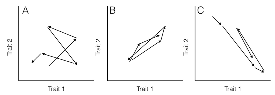
Figure 5.2. Hypothetical pathways of evolution (arrows) for (A) two uncorrelated traits, (B) two traits evolving with a positive covariance, and (C) two traits evolving with a negative covariance. Note that in (B), when trait 1 gets larger trait 2 also gets larger, but in (C) positive changes in trait 1 are paired with negative changes in trait 2. Image by the author, can be reused under a CC-BY-4.0 license.
When you have data for multiple continuous characters across many species along with a phylogenetic tree, you can fit a multivariate Brownian motion model to the data, as discussed in Chapter 3.
To calculate the likelihood, we can use the fact that, under our multivariate Brownian motion model, the joint distribution of all traits across all species has a multivariate normal distribution. Following Chapter 3, we find the variance-covariance matrix that describes that model by combining the two matrices R and C into a single large matrix using the Kroeneker product:
(eq. 5.3)
V = R ⊗ C
This matrix V is nr × nr. We can then substitute V for C in equation (4.5) to calculate the likelihood:
(eq. 5.4)
$$
L(\mathbf{x}_{nr} | \mathbf{a}, \mathbf{R}, \mathbf{C}) =
\frac
{e^{-1/2 (\mathbf{x}_{nr}- \mathbf{D} \cdot \mathbf{a})^\intercal (\mathbf{V})^{-1} (\mathbf{x}_nr-\mathbf{D} \cdot \mathbf{a})}}
{\sqrt{(2 \pi)^{nm} det(\mathbf{V})}}
$$
Here D is an nr × r design matrix where each element Dij is 1 if (j − 1)⋅n < i ≤ j ⋅ n and 0 otherwise. xnr is a single vector with all trait values for all species, listed so that the first n elements in the vector are trait 1, the next n are for trait 2, and so on:
(eq. 5.5)
$$
\mathbf{x}_{nr} =
\begin{bmatrix}
x_{11} & x_{12} & \dots & x_{1n} & x_{21} & \dots & x_{nr}\\
\end{bmatrix}
$$
We can find the value of the likelihood at its maximum by calculating L(xnr|a, R, C) using eq. 5.4 and an optimization routine to find the MLE.
Alternatively, one can calculate this MLE solution directly. Equations for estimating $\hat{\mathbf{a}}$ (the estimated vector of phylogenetic means for all characters) and $\hat{\mathbf{R}}$ (the estimated evolutionary rate matrix) are (Revell and Harmon 2008, Hohenlohe and Arnold (2008)):
(eq. 5.6)
$$
\hat{\mathbf{a}} = [(\mathbf{1}^\intercal \mathbf{C}^{-1} \mathbf{1})^{-1}(\mathbf{1}^\intercal \mathbf{C}^{-1} \mathbf{X})]^\intercal
$$
$$
\hat{\mathbf{R}} = \frac{(\mathbf{X} - \mathbf{1} \mathbf{\hat{a}})^\intercal \mathbf{C}^{-1} (\mathbf{X} - \mathbf{1} \mathbf{\hat{a}})}{n}
$$
Note here that we use X to denote the n (species) × r (traits) matrix of all traits across all species. Note the similarity between these multivariate equations (5.6 and 5.7) and their univariate equivalents (equations 4.6 and 4.7).
Section 5.4: Testing for evolutionary correlations
There are many ways to test for evolutionary correlations between two characters. Traditional methods like PICs and PGLS work great for testing evolutionary regression, which is very similar to testing for evolutionary correlations. However, when using those methods the connection to actual models of character evolution can remain opaque. Thus, I will first present approaches to test for correlated evolution based on model selection using AIC and Bayesian analysis. I will then return to “standard” methods for evolutionary regression at the end of the chapter.
Section 5.4a: Testing for character correlations using maximum likelihood and AIC
To test for an evolutionary correlation between two characters, we are really interested in the elements in the matrix R. For two characters, x and y, R can be written as:
(eq. 5.8)
$$
\mathbf{R} =
\begin{bmatrix}
\sigma_x^2 & \sigma_{xy} \\
\sigma_{xy} & \sigma_y^2 \\
\end{bmatrix}
$$
We are interested in the parameter σxy - the evolutionary covariance - and whether it is equal to zero (no correlation) or not. One simple way to test this hypothesis is to set up two competing hypotheses and compare them to each other. One hypothesis (H1) is that the traits evolve independently of each other, and another (H2) that the traits evolve with some covariance σxy. We can write these two rate matrices as:
(eq. 5.9)
$$
\begin{array}{lcr}
\mathbf{R}_{H_1} =
\begin{bmatrix}
\sigma_x^2 & 0 \\
0 & \sigma_y^2 \\
\end{bmatrix} &
\mathbf{R}_{H_2} =
\begin{bmatrix}
\sigma_x^2 & \sigma_{xy} \\
\sigma_{xy} & \sigma_y^2 \\
\end{bmatrix}\\
\end{array}
$$
We can calculate an ML estimate of the parameters in RH2 using equation 5.4. The maximum likelihood estimate of RH1 can be obtained by noting that, if character evolution is independent across all characters, then both σx2 and σy2 can be obtained by treating each character separately and using equations from chapter 3 to solve for each. It turns out that the ML estimates for σx2 and σy2 are always exactly the same for H1 and H2.
To compare these two models, we calculate the likelihood of each using equation 5.4. We can then compare these two likelihoods using either a likelihood ratio test or by comparing AICc scores (see chapter 2).
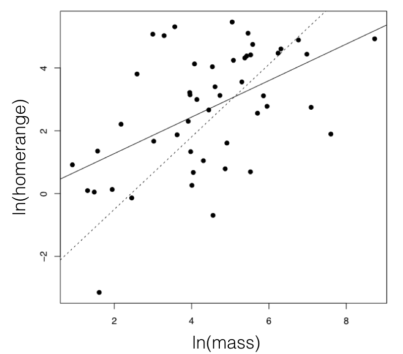
Figure 5.3. The relationship between mammal body mass and home-range size. To illustrate the effect of accounting for a tree, I plot a solid line for the regression line from a standard analysis, and dotted line from PGLS, which uses the phylogenetic tree. These methods are discussed in more detail in the next section. Image by the author, can be reused under a CC-BY-4.0 license.
For the mammal example, we can consider the two traits of (ln-transformed) body size and home range size (Garland 1992). These two characters have a positive correlation using standard regression analysis (r = 0.27), and a linear regression is significant (P = 0.0001; Figure 5.3). If we fit a multivariate Brownian motion model to these data, considering home range as trait 1 and body mass as trait 2, we obtain the following parameter estimates:
(eq. 5.10)
$$
\begin{array}{cc}
\hat{\mathbf{a}}_{H_2} =
\begin{bmatrix}
2.54 \\
4.64 \\
\end{bmatrix} &
\hat{\mathbf{R}}_{H_2} =
\begin{bmatrix}
0.24 & 0.10 \\
0.10 & 0.09 \\
\end{bmatrix}\\
\end{array}
$$
Note the positive off-diagonal element in the estimated R matrix, suggesting a positive evolutionary correlation between these two traits. This model corresponds to hypothesis 2 above, and has a log-likelihood of lnL = −164.0. If we fit a model with no correlation between the two traits, we obtain:
(eq. 5.11)
$$
\begin{array}{cc}
\hat{\mathbf{a}}_{H_1} =
\begin{bmatrix}
2.54 \\
4.64 \\
\end{bmatrix} &
\hat{\mathbf{R}}_{H_1} =
\begin{bmatrix}
0.24 & 0 \\
0 & 0.09 \\
\end{bmatrix}\\
\end{array}
$$
It is worth noting again that only the estimates of the evolutionary correlation were affected by this model restriction; all other parameter estimates remain the same. This model has a smaller (more negative) log-likelihood of lnL = −180.5.
A likelihood ratio test gives Δ = 33.0, and P < <0.001, rejecting the null hypothesis. The difference in AICc scores is 30.9, and the Akaike weight for model 2 is effectively 1.0. All ways of comparing these two models give strong support for hypothesis 2. We can conclude that there is an evolutionary correlation between body mass and home range size in mammals. What this means in evolutionary terms is that, across mammals, evolutionary changes in body mass tend to positively covary with changes in home range.
Section 5.4b: Testing for character correlations using Bayesian model selection
We can also implement a Bayesian approach to testing for the correlated evolution of two characters. The simplest way to do this is just to use the standard algorithm for Bayesian MCMC to fit a correlated model to the two characters. We can modify the algorithm presented in chapter 2 as follows:
- Sample a set of starting parameter values σx2, σy2, σxy, $\bar{z}_1(0)$, and $\bar{z}_2 (0)$ from prior distributions. For this example, we can set our prior distribution as uniform between 0 and 1 for σx2 and σy2, uniform from -1 to +1 for σxy, uniform from 1 to 9 for $\bar{z}_1(0)$ (lnMass), and -3 to 5 for $\bar{z}_1(0)$ (lnHomerange).
- Given the current parameter values, select new proposed parameter values using the proposal density Q(p′|p). Here, for all five parameter values, we will use a uniform proposal density with width 0.2, so that Q(p′|p)∼U(p − 0.1, p + 0.1).
- Calculate three ratios:
- The prior odds ratio, Rprior. This is the ratio of the probability of drawing the parameter values p and p’ from the prior. Since our priors are uniform, Rprior = 1.
- The proposal density ratio, Rproposal. This is the ratio of probability of proposals going from p to p’ and the reverse. Our proposal density is symmetrical, so that Q(p′|p)=Q(p|p′) and Rproposal = 1.
- The likelihood ratio, Rlikelihood. This is the ratio of probabilities of the data given the two different parameter values. We can calculate these probabilities from equation 5.6 above (eq. 5.12).
$$ R_{likelihood} = \frac{L(p'|D)}{L(p|D)} = \frac{P(D|p')}{P(D|p)} $$
- Find Raccept, the product of the prior odds, proposal density ratio, and the likelihood ratio. In this case, both the prior odds and proposal density ratios are 1, so Raccept = Rlikelihood.
- Draw a random number x from a uniform distribution between 0 and 1. If x < Raccept, accept the proposed value of all parameters; otherwise reject, and retain the current parameter values.
- Repeat steps 2-5 a large number of times.
We can then inspect the posterior distribution for the parameter is significantly greater than (or less than) zero. As an example, I ran this MCMC for 100,000 generations, discarding the first 10,000 generations as burn-in. I then sampled the posterior distribution every 100 generations, and obtained the following parameter estimates: $\hat{\sigma}_x^2 = 0.26$ [95% credible interval (CI): 0.18 - 0.38], $\hat{\sigma}_y^2 = 0.10$ (95% CI: 0.06 -0.15), and $\hat{\sigma}_{xy} = 0.11$ (95% CI: 0.06 - 0.17; see Figure 5.4). These results are comparable to our ML estimates. Furthermore, the 95% CI for σxy does not overlap with 0; in fact, none of the 901 posterior samples of σxy are less than zero. Again, we can conclude with confidence that there is an evolutionary correlation between these two characters.
Section 5.5c: Testing for character correlations using traditional approaches (PIC, PGLS)
The approach outlined above, which tests for an evolutionary correlation among characters using model selection, is not typically applied in the comparative biology literature. Instead, most tests of character correlation rely on phylogenetic regression using one of two methods: phylogenetic independent contrasts (PICs) and phylogenetic general least squares (PGLS). PGLS is actually mathematically identical to PICs in the simple case described here, and more flexible than PICs for other models and types of characters. Here I will review both PICs and PGLS and explain how they work and how they relate to the models described above.
Phylogenetic independent contrasts can be used to carry out a regression test for the relationship between two different characters. To do this, one calculates standardized PICs for trait x and trait y. One then uses standard linear regression forced through the origin to test for a relationship between these two sets of PICs. It is necessary to force the regression through the origin because the direction of subtraction of contrasts across any node in the tree is arbitrary; a reflection of all of the contrasts across both axes simultaneously should have no effect on the analyses3.
For mammal homerange and body mass, a PIC regression test shows a significant correlation between the two traits (P < <0.0001; Figure 5.5).
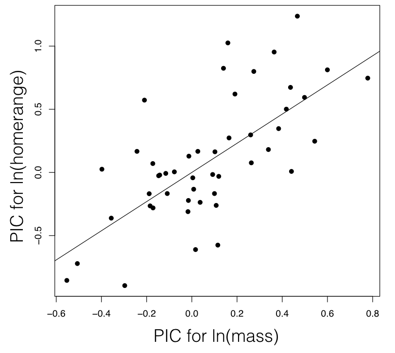
Figure 5.4. Regression based on independent contrasts. The regression line is forced through the origin. Image by the author, can be reused under a CC-BY-4.0 license.
There is one drawback to PIC regression analysis, though – one does not recover an estimate of the intercept of the regression of y on x – that is, the value of y one would expect when x = 0. The easiest way to get this parameter estimate is to instead use Phylogenetic Generalized Least Squares (PGLS). PGLS uses the common statistical machinery of generalized least squares, and applies it to phylogenetic comparative data. In normal generalized least squares, one constructs a model of the relationship between y and x, as:
(eq. 5.13)
y = XDb + ϵ
Here, y is an n × 1 vector of trait values and b is a vector of unknown regression coefficients that must be estimated from the data. XD is a design matrix including the traits that one wishes to test for a correlation with y and – if the model includes an intercept – a column of 1s. To test for correlations, we use:
(eq. 5.14)
$$
\mathbf{X_D} =
\begin{bmatrix}
1 & x_1 \\
1 & x_2 \\
\dots & \dots \\
1 & x_n \\
\end{bmatrix}
$$
In the case of one predictor and one response variable, b is 2 × 1 and the resulting model can be used to test correlations between two characters. However, XD could also be multivariate, and can include more than one character that might be related to y. This allows us to carry out the equivalent of multiple regression in a phylogenetic context. Finally, ϵ are the residuals – the difference between the y-values predicted by the model and their actual values. In traditional regression, one assumes that the residuals are all normally distributed with the same variance. By contrast, with GLS, one assumes that the residuals might not be independent of each other; instead, they are multivariate normal with expected mean zero and some variance-covariance matrix Ω.
In the case of Brownian motion, we can model the residuals as having variances and covariances that follow the structure of the phylogenetic tree. In other words, we can substitute our phylogenetic variance-covariance matrix C as the matrix Ω. We can then carry out standard GLS analyses to estimate model parameters:
(eq. 5.15)
$$
\hat{\mathbf{b}} = (\mathbf{X}_D ^ \intercal \mathbf{\Omega}^{-1} \mathbf{X}_D ^ \intercal)^{-1} \mathbf{X}_D ^ \intercal \mathbf{\Omega}^{-1} \mathbf{y} = (\mathbf{X}_D ^ \intercal \mathbf{C}^{-1} \mathbf{X}_D ^ \intercal)^{-1} \mathbf{X}_D ^ \intercal \mathbf{C}^{-1} \mathbf{y}
$$
The first term in $\hat{\mathbf{b}}$ is the phylogenetic mean $\bar{z}(0)$. The other term in $\hat{\mathbf{b}}$ will be an estimate for the slope of the relationship between y and x, the calculation of which statistically controls for the effect of phylogenetic relationships.
Applying PGLS to mammal body mass and home range results in an identical estimate of the slope and P-value as we obtain using independent contrasts. PGLS also returns an estimate of the intercept of this relationship, which cannot be obtained from the PICs.
Of course, another difference is that PICs and PGLS use regression, while the approach outlined above tests for a correlation. These two types of statistical tests are different. Correlation tests for a relationship between x and y, while regression tries to find the best way to predict y from x. For correlation, it does not matter which variable we call x and which we call y. However, in regression we will get a different slope if we predict y given x instead of predicting x given y. The model that is assumed by phylogenetic regression models is also different from the model above, where we assumed that the two characters evolve under a correlated Brownian motion model. By contrast, PGLS (and, implicitly, PICs) assume that the deviations of each species from the regression line evolve under a Brownian motion model. We can imagine, for example, that species can freely slide along the regression line, but that evolving around that line can be captured by a normal Brownian model. Another way to think about a PGLS model is that we are treating x as a fixed property of species. The deviation of y from what is predicted by x is what evolves under a Brownian motion model. If this seems strange, that’s because it is! There are other, more complex models for modeling the correlated evolution of two characters that make assumptions that are more evolutionarily realistic (e.g. Hansen 1997); we will return to this topic later in the book. At the same time, PGLS is a well-used method for evolutionary regression, and is undoubtedly useful despite its somewhat strange assumptions.
PGLS analysis, as described above, assumes that we can model the error structure of our linear model as evolving under a Brownian motion model. However, one can change the structure of the error variance-covariance matrix to reflect other models of evolution, such as Ornstein-Uhlenbeck. We return to this topic in a later chapter.
Section 5.6: Summary
There are at least four methods for testing for an evolutionary correlation between continuous characters: likelihood ratio test, AIC model selection, PICs, and PGLS. These four methods as presented all make the same assumptions about the data and, therefore, have quite similar statistical properties. For example, if we simulate data under a multivariate Brownian motion model, both PICs and PGLS have appropriate Type I error rates and very similar power. Any of these are good choices for testing for the presence of an evolutionary correlation in your data.
Section 5.7: Footnotes
1: We might also want to carry out linear regression, which is related to correlation analysis but distinct. We will show examples of phylogenetic regression at the end of this chapter.
2: Although the joint distribution of all species for a single trait is multivariate normal (see previous chapters), individual changes along a particular branch of a tree are univariate.
3: Another way to think about regression through the origin is to think of pairs of contrasts across any node in the tree as two-dimensional vectors. Calculating a vector correlation is equivalent to calculating a regression forced through the origin.
References
Felsenstein, J. 1985. Phylogenies and the comparative method. Am. Nat. 125:1–15.
Garland, T., Jr. 1992. Rate tests for phenotypic evolution using phylogenetically independent contrasts. Am. Nat. 140:509–519.
Hansen, T. F. 1997. Stabilizing selection and the comparative analysis of adaptation. Evolution 51:1341–1351.
Hohenlohe, P. A., and S. J. Arnold. 2008. MIPoD: A hypothesis-testing framework for microevolutionary inference from patterns of divergence. Am. Nat. 171:366–385.
Revell, L. J., and L. J. Harmon. 2008. Testing quantitative genetic hypotheses about the evolutionary rate matrix for continuous characters. Evol. Ecol. Res. 10:311–331.