Phylogenetic Comparative Methods learning from trees
- Chapter 10: Introduction to birth-death models
- Section 10.1: Plant diversity imbalance
- Section 10.2: The birth-death model
- Section 10.3: Birth-death models and phylogenetic trees
- Section 10.4: Simulating birth-death trees
- Section 10.5: Tree topology, tree shape, and tree balance under a birth-death model
- Section 10.6: Lineage-through-time plots
- Section 10.7: Chapter Summary
Chapter 10: Introduction to birth-death models
Section 10.1: Plant diversity imbalance
The diversity of flowering plants (the angiosperms) dwarfs the number of species of their closest evolutionary relatives (Figure 10.1). There are more than 260,000 species of angiosperms (that we know; more are added every day). The clade originated more than 140 million years ago (Bell et al. 2005), and all of these species have formed since then. One can contrast the diversity of angiosperms with the diversity of other groups that originated at around the same time. For example, gymnosperms, which are as old as angiosperms, include only around 1000 species, and may even represent more than one clade. The diversity of angiosperms also dwarfs the diversity of familiar vertebrate groups of similar age (e.g. squamates - snakes and lizards - which diverged from their sister taxon, the tuatara, some 250 mya or more Hedges et al. 2006, include fewer than 8000 species).
The evolutionary rise of angiosperm diversity puzzled Darwin over his career, and the issues surrounding angiosperm diversification are often referred to as “Darwin’s abominable mystery” in the scientific literature (e.g. Davies et al. 2004). The main mystery is the tremendous variation in numbers of species across plant clades (see Figure 10.1). This variation even applies within angiosperms, where some clades are much more diverse than others.
At a global scale, the number of species in a clade can change only via two processes: speciation and extinction. This means that we must look to speciation and extinction rates – and how they vary through time and across clades – to explain phenomena like the extraordinary diversity of Angiosperms. It is to this topic that we turn in the next few chapters. Since Darwin’s time, we have learned a lot about the evolutionary processes that led to the diversity of angiosperms that we see today. These data provide an incredible window into the causes and effects of speciation and extinction over macroevolutionary time scales.
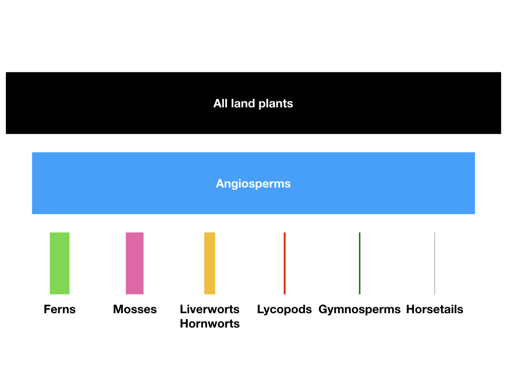
Figure 10.1. Diversity of major groups of embryophytes (land plants); bar areas are proportional to species diversity of each clade. Angiosperms, including some 250,000 species, comprise more than 90% of species of land plants. Figure inspired by Crepet and Niklas (2009). Image by the author, can be reused under a CC-BY-4.0 license.
Comparative methods can be applied to understand patterns of species richness by estimating speciation and extinction rates, both across clades and through time. In this chapter, I will introduce birth-death models, by far the most common model for understanding diversification in a comparative framework. I will discuss the mathematics of birth-death models and how these models relate to the shapes of phylogenetic trees. I will describe how to simulate phylogenetic trees under a birth-death model. Finally, I will discuss tree balance and lineage-through-time plots, two common ways to measure the shapes of phylogenetic trees.
Section 10.2: The birth-death model
A birth-death model is a continuous-time Markov process that is often used to study how the number of individuals in a population change through time. For macroevolution, these “individuals” are usually species, sometimes called "lineages" in the literature. In a birth-death model, two things can occur: births, where the number of individuals increases by one; and deaths, where the number of individuals decreases by one. We assume that no more than one new individual can form (or die) during any one event. In phylogenetic terms, that means that birth-death trees cannot have “hard polytomies” - each speciation event results in exactly two descendant species.
In macroevolution, we apply the birth-death model to species, and typically consider a model where each species has a constant probability of either giving birth (speciating) or dying (going extinct). We denote the per-lineage birth rate as λ and the per-lineage death rate as μ. For now we consider these rates to be constant, but we will relax that assumption later in the book.
We can understand the behavior of birth-death models if we consider the waiting time between successive speciation and extinction events in the tree. Imagine that we are considering a single lineage that exists at time t0. We can think about the waiting time to the next event, which will either be a speciation event splitting that lineage into two (Figure 10.2A) or an extinction event marking the end of that lineage (Figure 10.2B). Under a birth-death model, both of these events follow a Poisson process, so that the expected waiting time to an event follows an exponential distribution (Figure 10.2C). The expected waiting time to the next speciation event is exponential with parameter λ, and the expected waiting time to the next extinction event exponential with parameter μ. [Of course, only one of these can be the next event. The expected waiting time to the next event (of any sort) is exponential with parameter λ + μ, and the probability that that event is speciation is λ/(μ + λ), extinction μ/(μ + λ)].
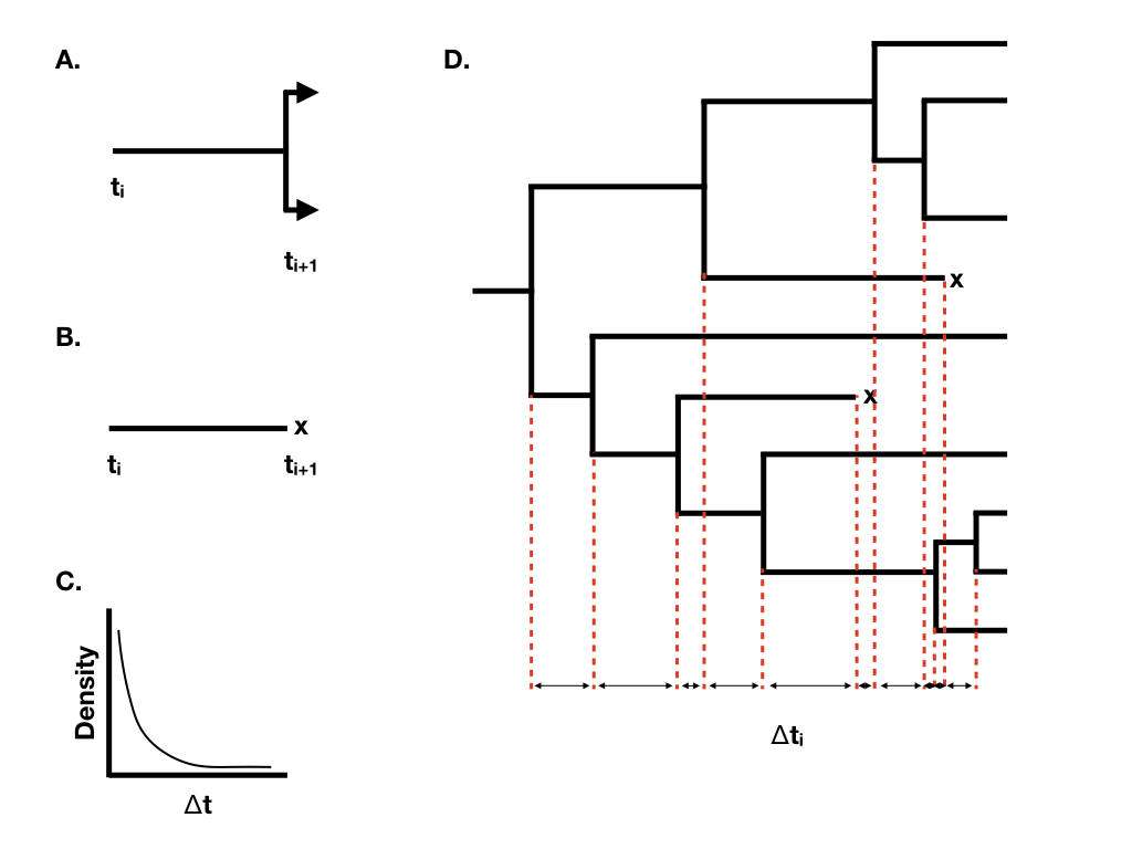
Figure 10.2. Illustration of the basic properties of birth-death models. A. Waiting time to a speciation event; B. Waiting time to an extinction event; C. Exponential distribution of waiting times until the next event; D. A birth-death tree with waiting times, with x denoting extinct taxa. Image by the author, can be reused under a CC-BY-4.0 license.
When we have more than one lineage “alive” in the tree at any time point, then the waiting time to the next event changes, although its distribution is still exponential. In general, if there are N(t) lineages alive at time t, then the waiting time to the next event follows an exponential distribution with parameter N(t)(λ + μ), with the probability that that event is speciation or extinction the same as given above. You can see from this equation that the rate parameter of the exponential distribution gets larger as the number of lineages increases. This means that the expected waiting times across all lineages get shorter and shorter as more lineages accumulate.
Using this approach, we can grow phylogenetic trees of any size (Figure 10.2D).
We can derive some important properties of the birth-death process on trees. To do so, it is useful to define two additional parameters, the net diversification rate (r) and the relative extinction rate (ϵ):
(eq. 10.1)
r = λ − μ
$$
\epsilon = \frac{\mu}{\lambda}
$$
These two parameters simplify some of the equations below, and are also commonly encountered in the literature.
To derive some general properties of the birth-death model, we first consider the process over a small interval of time, Δt. We assume that this interval is so short that it contains at most a single event, either speciation or extinction (the interval might also contain no events at all). The probability of speciation and extinction over the time interval can be expressed as:
(eq. 10.2)
Prspeciation = N(t)λΔt
Prextinction = N(t)μΔt
We now consider the total number of living species at some time t, and write this as N(t). It is useful to think about the expected value of N(t) under a birth-death model [we consider the full distribution of N(t) below]. The expected value of N(t) after a small time interval Δt is:
(eq. 10.3)
N(t + Δt)=N(t)+N(t)λΔt − N(t)μΔt
We can convert this to a differential equation by subtracting N(t) from both sides, then dividing by Δt and taking the limit as Δt becomes very small:
(eq. 10.4)
dN/dt = N(λ − μ)
We can solve this differential equation if we set a boundary condition that N(0)=n0; that is, at time 0, we start out with n0 lineages. We then obtain:
(eq. 10.5)
N(t)=n0eλ − μt = n0ert
This deterministic equation gives us the expected value for the number of species through time under a birth-death model. Notice that the number of species grows exponentially through time as long as λ > μ, i.e. r > 0, and decays otherwise (Figure 10.3).
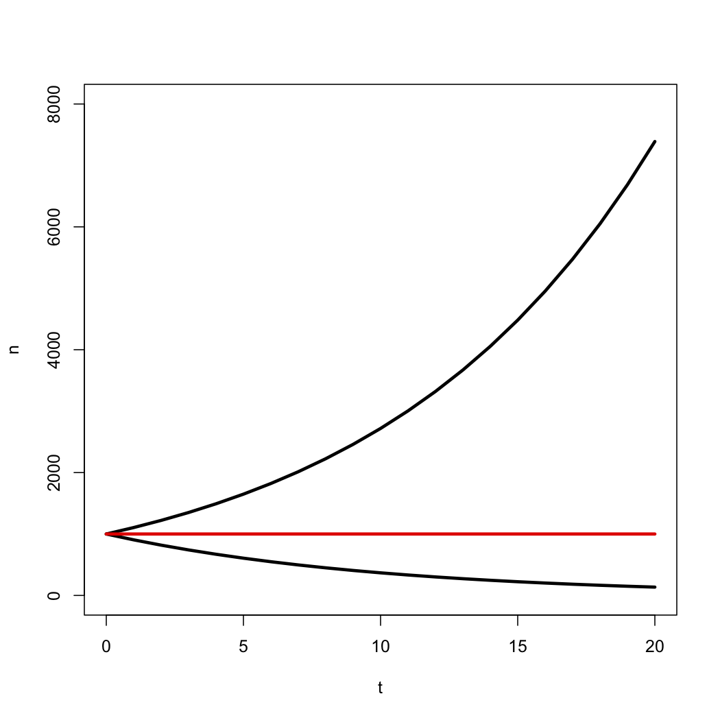
Figure 10.3. Expected number of species under a birth-death model with r = λ − μ > 0 (top line), r = 0 (middle line), and r < 0 (bottom line). In each case the starting number of species was n0 = 1000. Image by the author, can be reused under a CC-BY-4.0 license.
We are also interested in the stochastic behavior of the model – that is, how much should we expect N(t) to vary from one replicate to the next? We can calculate the full probability distribution for N(t), which we write as pn(t)=Pr[N(t)=n] for all n ≥ 0, to completely describe the birth-death model’s behavior. To derive this probability distribution, we can start with a set of equations, one for each value of n, to keep track of the probabilities of n lineages alive at time t. We will denote each of these as pn(t) (there are an infinite set of such equations, from p0 to p∞). We can then write a set of difference equations that describe the different ways that one can reach any state over some small time interval Δt. We again assume that Δt is sufficiently small that at most one event (a birth or a death) can occur. As an example, consider what can happen to make n = 0 at the end of a certain time interval. There are two possibilities: either we were already at n = 0 at the beginning of the time interval and (by definition) nothing happened, or we were at n = 1 and the last surviving lineage went extinct. We write this as:
(eq. 10.6)
p0(t + Δt)=p1(t)μΔt + p0(t)
Similarly, we can reach n = 1 by either starting with n = 1 and having no events, or going from n = 2 via extinction.
(eq. 10.7)
p1(t + Δt)=p1(t)(1 − (λ + μ))Δt + p2(t)2μΔt
Finally, any for n > 1, we can reach the state of n lineages in three ways: from a birth (from n − 1 to n), a death (from n + 1 to n), or neither (from n to n).
(eq. 10.8)
pn(t + Δt)=pn − 1(t)(n − 1)λΔt + pn + 1(t)(n + 1)μΔt + pn(t)(1 − n(λ + μ))Δt
We can convert this set of difference equations to differential equations by subtracting pn(t) from both sides, then dividing by Δt and taking the limit as Δt becomes very small. So, when n = 0, we use 10.6 to obtain:
(eq. 10.9)
dp0(t)/dt = μp1(t)
From 10.7:
(eq. 10.10)
dp1(t)/dt = 2μp2(t)−(λ − μ)p1(t)
and from 10.8, for all n > 1:
(eq. 10.11)
dpn(t)/dt = (n − 1)λpn − 1(t)+(n + 1)μpn + 1(t)−n(λ + μ)pn(t)
We can then solve this set of differential equations to obtain the probability distribution of pn(t). Using the same boundary condition, N(0)=n0, we have p0(t)=1 for n = n0 and 0 otherwise. Then, we can find the solution to the differential equations 10.9, 10.10, and 10.11. The derivation of the solution to this set of differential equations is beyond the scope of this book (but see Kot 2001 for a nice explanation of the mathematics). A solution was first obtained by Bailey (1964), but I will use the simpler equivalent form from Foote et al. (1999). For p0(t) – that is, the probability that the entire lineage has gone extinct at time t – we have:
(eq. 10.12)
p0(t)=α0n
And for all n ≥ 1:
(eq. 10.13)
$$
p_n(t) = \sum\limits_{j=1}^{min(n_0,n)} \binom{n_0}{j} \binom{n-1}{j-1} \alpha^{n_0 - j} \beta^{n-j} [(1-\alpha)(1-\beta)]^j
$$
Where α and β are defined as:
(eq. 10.14)
$$
\alpha=\frac{\epsilon (e^rt-1)}{(e^rt-\epsilon)}
$$
$$
\beta =\frac{(e^rt-1)}{(e^rt-\epsilon)}
$$
α is the probability that any particular lineage has gone extinct before time t.
Note that when n0 = 1 – that is, when we start with a single lineage - equations 10.12 and 10.13 simplify to (Raup 1985):
(eq. 10.15)
p0(t)=α
And for all n ≥ 1:
(eq. 10.16)
pn(t)=(1 − α)(1 − β)βi − 1
In all cases the expected number of lineages in the tree is exactly as stated above in equation (10.5), but now we have the full probability distribution of the number of lineages given n0, t, λ, and μ. A few plots capture the general shape of this distribution (Figure 10.4).
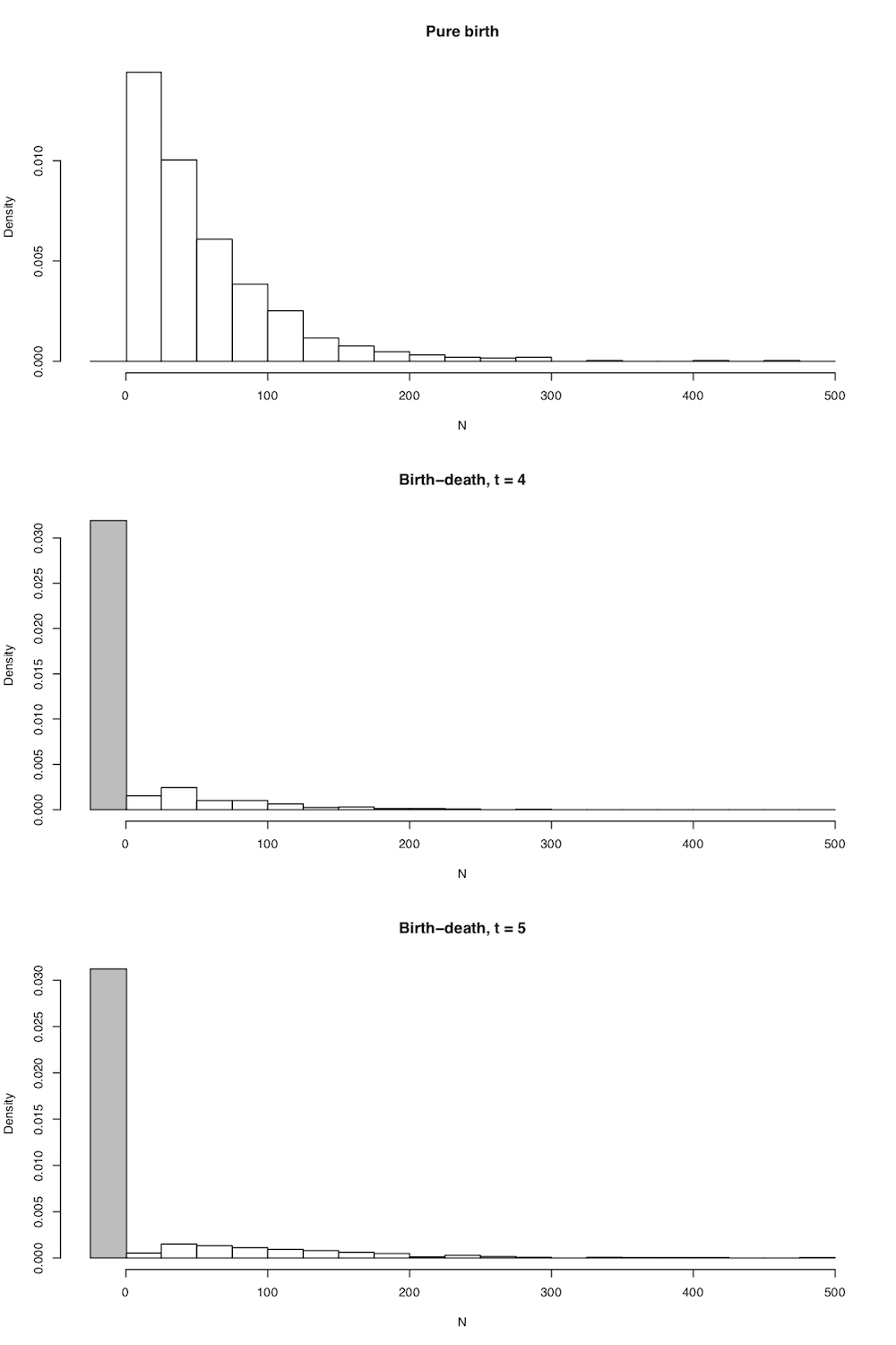
Figure 10.4. Probability distributions of N(t) under A. pure birth, B. birth death after a short time, and C. birth-death after a long time. Image by the author, can be reused under a CC-BY-4.0 license.
There are quite a few comparative methods that use clade species richness and age along with the distributions defined in 10.14 and 10.15 to make inferences about clade diversification rates (see chapter 11).
Section 10.3: Birth-death models and phylogenetic trees
The above discussion considered the number of lineages under a birth-death model, but not their phylogenetic relationships. However, just by keeping track of the parent-offspring relationships among lineages, we can consider birth-death models that result in phylogenetic trees (e.g. Figure 10.2D).
The main complication in phylogenetic studies of birth-death models is that we get a “censored” view of the process, in that we only observe lineages that survive to the present day. In the above example, if the true phylogenetic tree were the one plotted in 10.5A, we would only have a chance to observe the phylogenetic tree in figure 10.5B – and even then only if we sampled all of the species and reconstructed the tree with perfect accuracy! A partially sampled tree with only extant species can be seen in Figure 10.5C. I will cover the relationship between birth-death models and the branch lengths of phylogenetic trees in much more detail in the next chapter.
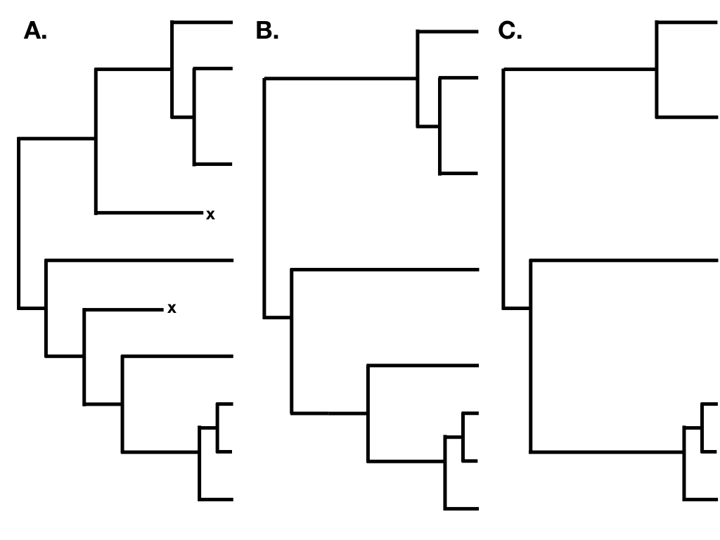
Figure 10.5. A. A birth-death tree including all extinct and extant species; B. A birth-death tree including only extant species; and C. A partially sampled birth-death tree including only some extant species. Image by the author, can be reused under a CC-BY-4.0 license.
Section 10.4: Simulating birth-death trees
We can use the statistical properties of birth-death models to simulate phylogenetic trees through time. We could begin with a single lineage at time 0. However, phylogenetic tree often start with the first speciation event in the clade, so one can also begin the simulation with two lineages at time 0 (this difference relates to the distinction between crown and stem ages of clades; see also Chapter 11).
To simulate our tree, we need to draw waiting times between speciation and extinction events, connect new lineages to the tree, and prune lineages when they go extinct. We also need a stopping criterion, which can have to do with a particular number of taxa or a fixed time interval. We will consider the latter, and leave growing trees to a fixed number of taxa as an exercise for the reader. Our simulation algorithm is as follows. I assume that we have a certain number of “living” lineages in our tree (1 or 2 initially), a current time (tc = 0 initially), and a stopping time tstop.
- Draw a waiting time ti to the next speciation or extinction event. Waiting times are drawn from an exponential distribution with rate parameter Nalive * (λ + μ) where Nalive is the current number of living lineages in the tree.
- Check to see if the simulation ends before the next event. That is, if tc + ti > tstop, end the simulation.
- Decide whether the next event is a speciation event [with probability λ/(λ + μ)] or an extinction event [with probability μ/(λ + μ)]. This can be done by drawing a uniform random number ui from the interval [0, 1] and assigning speciation to the event if ui < λ/(λ + μ) and extinction otherwise.
- If (3) is a speciation event, then choose a random living lineage in the tree. Attach a new branch to the tree at this point, and add one new living lineage to the simulation. Return to step 1.
- If (3) is an extinction event, choose a random living lineage in the tree. That lineage is now dead. As long as there is still at least one living lineage in the tree, return to (1); otherwise, your whole clade has gone extinct, and you can stop the simulation.
This procedure returns a phylogenetic tree that includes both living and dead lineages. One can prune out any extinct taxa to return a birth-death tree of survivors, which is more in line with what we typically study using extant species. It is also worth noting that entire clades can – and often do – go extinct under this protocol before one reaches time tstop. Note also that there is a much more efficient way to simulate trees (Stadler 2011).
We can think about phylogenetic predictions of birth-death models in two ways: by considering tree topology, and by considering tree branch lengths. I will consider each of these two aspects of trees below.
Section 10.5: Tree topology, tree shape, and tree balance under a birth-death model
Tree topology summarizes the patterns of evolutionary relatedness among a group of species independent of the branch lengths of a phylogenetic tree. Two different trees have the same topology if they define the exact same set of clades. This is important because sometimes two trees can look very different and yet still have the same topology (e.g. Figure 10.6 A, B, and C).
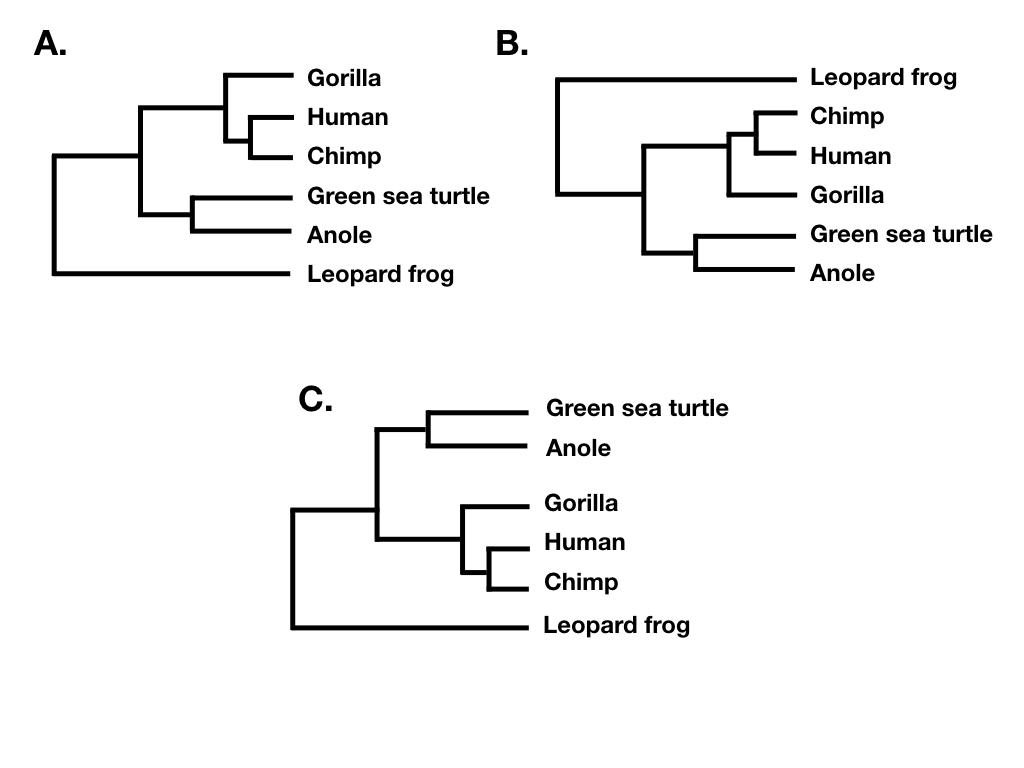
Figure 10.6. Several phylogenetic trees showing different ways to plot the same tree topology. Image by the author, can be reused under a CC-BY-4.0 license.
Tree shape ignores both branch lengths and tree tip labels. For example, the two trees in figure 10.7 A and B have the same tree shape even though they share no tips in common. What they do share is that their nodes have the same patterns in terms of the number of descendants on each “side” of the bifurcation. By contrast, the phylogenetic tree in 10.7 C has a different shape. (Note that what I am calling tree shape is sometimes referred to as “unlabeled” tree topology; e.g. Felsenstein 2004).
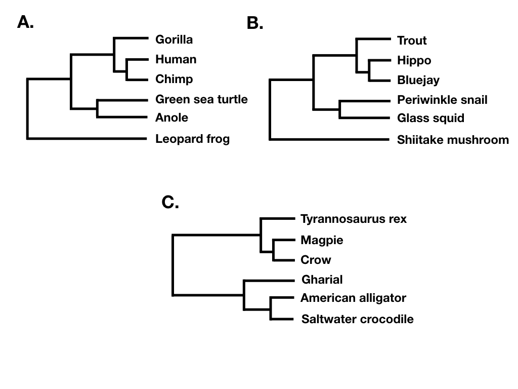
Figure 10.7. Two different phylogenetic trees sharing the same tree shape (A and B), and one with a different shape (C). Image by the author, can be reused under a CC-BY-4.0 license.
Finally, tree balance is a way of expressing differences in the number of descendants between pairs of sister lineages at different points in a phylogenetic tree. For example, consider the phylogenetic tree depicted in figure 10.7B. The deepest split in that tree separates a clade with five species (trout, hippo, bluejay, periwinkle snail, glass squid) from a clade with a single species (Shiitake mushroom), and so that node in the tree is unbalanced with a (5, 1) pattern. By contrast, the deepest split in 10.7C separates two clades of equal size. In that tree, the deepest node is balanced with a (3, 3) pattern. A number of approaches in macroevolution use balance at nodes and across whole trees to try to capture important evolutionary patterns.
We can start to understand these approaches by considering the balance of a single node n in a phylogenetic tree. There are two clades descended from this node; let’s call them a and b. We assume that the total number of species descended from the node Ntotal = Na + Nb is constant and that neither Na nor Nb is zero. An important result, first discussed by Farris (1976) for a pure-birth model, is that all possible numerical divisions of Ntotal into Na + Nb are equally probable. For example, if Ntotal = 10, then all possible divisions: 1 + 9, 2 + 8, 3 + 7, 4 + 6, 5 + 5, 6 + 4, 7 + 3, 8 + 2, and 9 + 1 are all equally probable, so that each will be predicted to occur with a probability 1/9. Formally,
(eq. 10.17)
$$
p(N_a \mid N_{total})=\frac{1}{N_{total}-1}
$$
Note that there is a subtle difference between equation 10.2 above and some equations in the literature, e.g. Slowinski and Guyer (1993). This difference has to do with whether we label the two descendent clades, a and b, or not; if the clades are unlabeled, then there is no difference between 4+6 and 6+4, so that the probability that the largest clade, whichever it might be, has 6 species is twice what is given by my equation.
Equation 10.17 applies even if there is extinction, as long as both sister clades have the same speciation and extinction rates (Slowinski and Guyer 1993). This equation has been used to compare diversification rates between sister clades, either for a single pair or across multiple pairs (see Chapter 11).
Tree balance statistics provide a way of comparing numbers of taxa across all of the nodes in a phylogenetic tree simultaneously. There are a surprisingly large number of tree balance statistics, but all rely on summarizing information about the balance of each node across a whole tree. Colless’ index Ic (Colless 1982) is one of the simplest – and, perhaps, most commonly used – indices of tree balance. Ic is the sum of the difference in the number of tips subtended on each side of every node in the tree, standardized by the maximum that such a sum can achieve:
(eq. 10.18)
$$
I_C = \frac{\sum\limits_{all nodes} (N_L - N_R)}{(N-1)(N-2)/2}
$$
If the tree is perfectly balanced (only possible when N is some power of 2, e.g. 2, 4, 8, 16, etc.), then IC = 0 (Figure 10.7C). By contrast, if the tree is completely pectinate, which means that each split in the tree contrasts a clade with 1 species with the rest of the species in the clade, then IC = 1 (Figure 10.7A). All phylogenetic trees have values of IC between 0 and 1 (Figure 10.7B).

Figure 10.8. A. a pectinate tree (IC = 1); B. a random tree (0 < IC < 1); C. A balanced tree (IC = 0). Image by the author, can be reused under a CC-BY-4.0 license.
There are a number of other indices of phylogenetic tree balance (reviewed in Mooers and Heard 1997). All of these indices are used in a similar way: one can then compare the value of the tree index to what one might expect under a particular model of diversification, typically birth-death. In fact, since these indices focus on tree topology and ignore branch lengths, one can actually consider their general behavior under a set of equal-rates Markov (ERM) models. This set includes any model where birth and death rates are equal across all lineages in a phylogenetic tree at a particular time. ERM models include birth-death models as described above, but also encompass models where birth and/or death rates change through time.
Section 10.6: Lineage-through-time plots
The other main way to quantify phylogenetic tree shape is by making lineage-through-time plots. These plots have time along the x axis (from the root of the tree to the present day), and the reconstructed number of lineages on the y-axis (Figure 10.8). Since we are usually considering birth-death models, where the number of lineages is expected to grow (or shrink) exponentially through time, then it is typical practice to log-transform the y-axis.
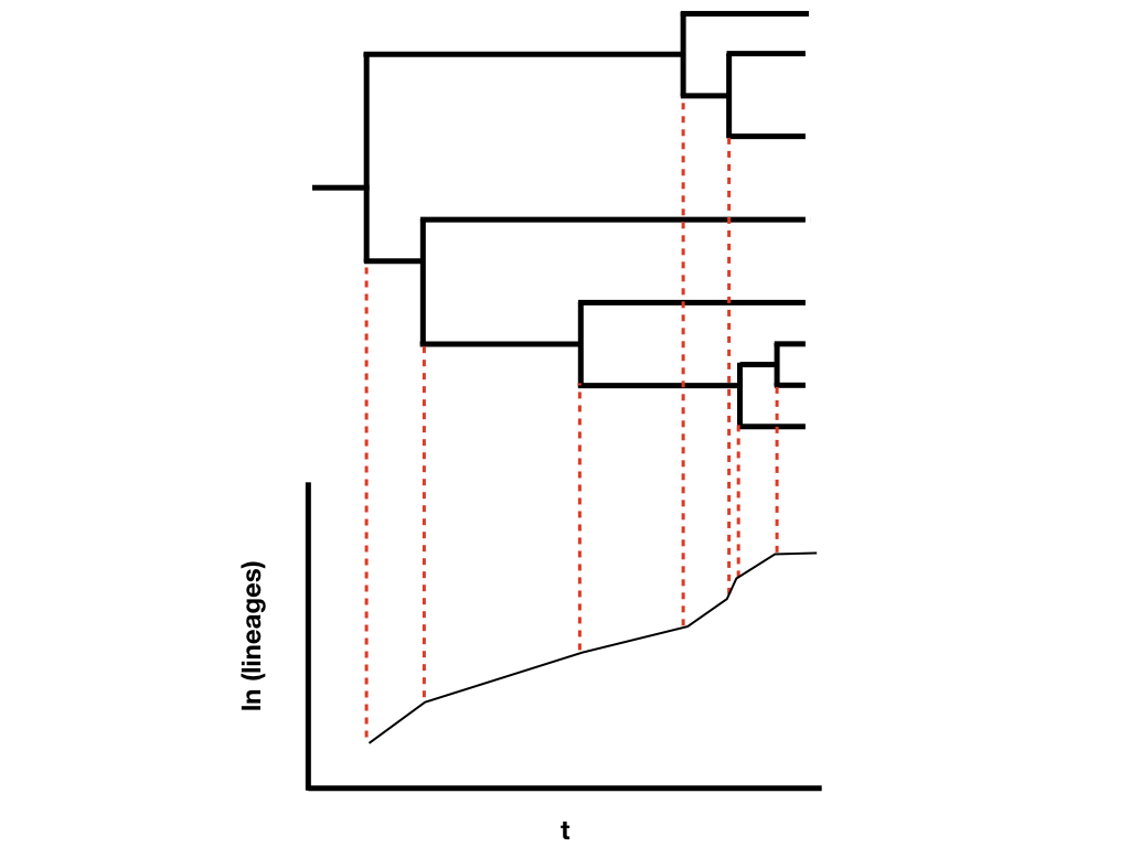
Figure 10.9. Lineage-through-time plot. Image by the author, can be reused under a CC-BY-4.0 license.
Lineage-through-time plots are effective ways to visualize patterns of lineage diversification through time. Under a pure-birth model on a semi-log scale, LTT plots follow a straight line on average (Figure 10.9A). By contrast, extinction should leave a clear signal in LTT plots because the probability of a lineage going extinct depends on how long it has been around; old lineages are much more likely to have been hit by extinction than relatively young lineages. We see this reflected in LTT plots as the “pull of the present” – an upturn in the slope of the LTT plot near the present day (Figure 10.9B). Incomplete sampling – that is, not sampling all of the living species in a clade – can also have a huge impact on the shape of LTT plots (Figure 10.9C). We will discuss LTT plots further in chapter 11, where we will use them to make inferences about patterns of lineage diversification through time.
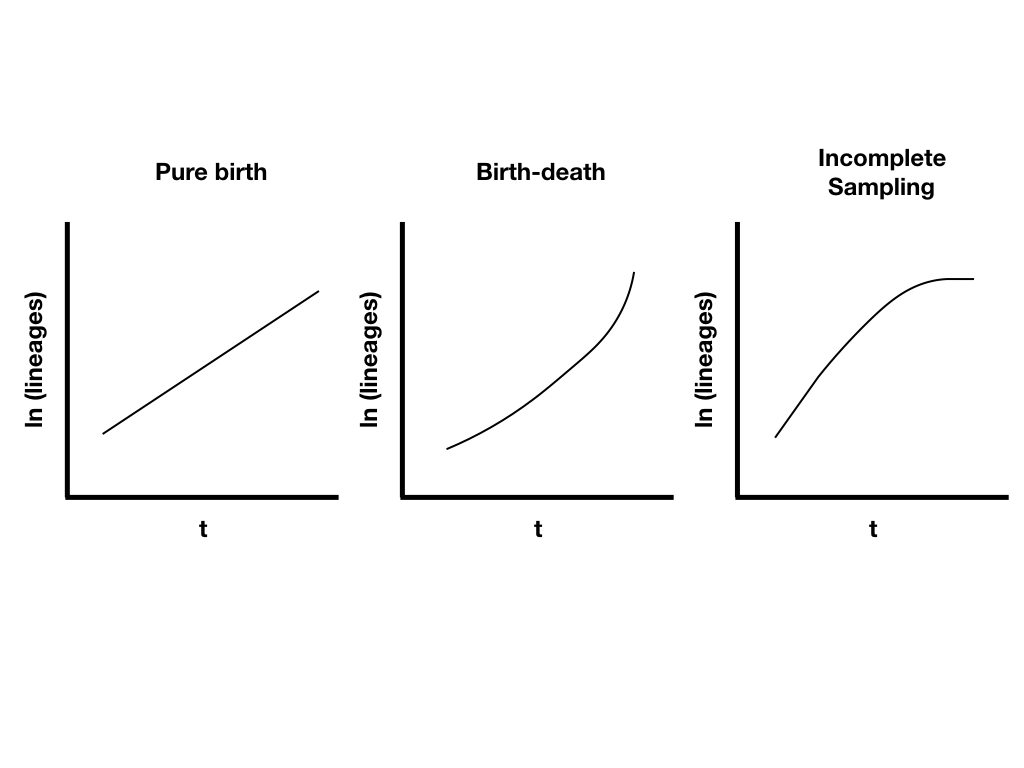
Figure 10.10. Example lineage-through-time plots. Image by the author, can be reused under a CC-BY-4.0 license.
Section 10.7: Chapter Summary
In this chapter, I introduced birth-death models and summarized their basic mathematical properties. Birth-death models predict patterns of species diversity over time intervals, and can also be used to model the growth of phylogenetic trees. We can visualize these patterns by measuring tree balance and creating lineage-through-time (LTT) plots.
References
Bailey, N. T. J. 1964. The elements of stochastic processes with applications to the natural sciences. John Wiley & Sons.
Bell, C. D., D. E. Soltis, and P. S. Soltis. 2005. The age of the angiosperms: A molecular timescale without a clock. Evolution 59:1245–1258.
Colless, D. H. 1982. Review of phylogenetics: The theory and practice of phylogenetic systematics. Syst. Zool.
Crepet, W. L., and K. J. Niklas. 2009. Darwin’s second “abominable mystery”: Why are there so many angiosperm species? Am. J. Bot. Botanical Soc America.
Davies, T. J., T. G. Barraclough, M. W. Chase, P. S. Soltis, D. E. Soltis, and V. Savolainen. 2004. Darwin’s abominable mystery: Insights from a supertree of the angiosperms. Proc. Natl. Acad. Sci. U. S. A. 101:1904–1909.
Farris, J. S. 1976. Expected asymmetry of phylogenetic trees. Syst. Zool. 25:196–198. [Oxford University Press, Society of Systematic Biologists, Taylor & Francis, Ltd.].
Felsenstein, J. 2004. Inferring phylogenies. Sinauer Associates, Inc., Sunderland, MA.
Foote, M., J. P. Hunter, C. M. Janis, and J. J. Sepkoski Jr. 1999. Evolutionary and preservational constraints on origins of biologic groups: Divergence times of eutherian mammals. Science 283:1310–1314.
Hedges, S. B., J. Dudley, and S. Kumar. 2006. TimeTree: A public knowledge-base of divergence times among organisms. Bioinformatics 22:2971–2972.
Kot, M. 2001. Stochastic birth and death processes. Pp. 25–42 in M. Kot, ed. Elements of mathematical ecology. Cambridge University Press, Cambridge.
Mooers, A. O., and S. B. Heard. 1997. Inferring evolutionary process from phylogenetic tree shape. Q. Rev. Biol. 72:31–54.
Raup, D. M. 1985. Mathematical models of cladogenesis. Paleobiology 11:42–52.
Slowinski, J. B., and C. Guyer. 1993. Testing whether certain traits have caused amplified diversification: An improved method based on a model of random speciation and extinction. Am. Nat. 142:1019–1024.
Stadler, T. 2011. Simulating trees with a fixed number of extant species. Syst. Biol. 60:676–684.