Phylogenetic Comparative Methods learning from trees
R markdown to recreate analyses
Chapter 7: Models of discrete character evolution
Section 7.1: Limblessness as a discrete trait
Squamates, the clade that includes all living species of lizards, are well known for their diversity. From the gigantic Komodo dragon of Indonesia (Figure 7.1A, Varanus komodoensis) to tiny leaf chameleons of Madagascar (Figure 7.1B, Brookesia), squamates span an impressive range of form and ecological niche use (Vitt et al. 2003; Pianka et al. 2017). Even the snakes (Figure 7.1C and D), extraordinarily diverse in their own right (~3,500 species), are actually a clade that is nested within squamates (Streicher and Wiens 2017). The squamate lineage that is ancestral to snakes became limbless about 170 million years ago (see Hedges et al. 2006) – and also underwent a suite of changes to their head shape, digestive tract, and other traits associated with their limbless lifestyle. In other words, snakes are lizards – highly modified lizards, but lizards nonetheless. And snakes are not the only limbless lineage of squamates. In fact, lineages within squamates have lost their limbs over and over again through their history (e.g. Figure 7.1E and F), with some estimates that squamates have lost their limbs at least 26 times in the past 240 million years (Brandley et al. 2008).
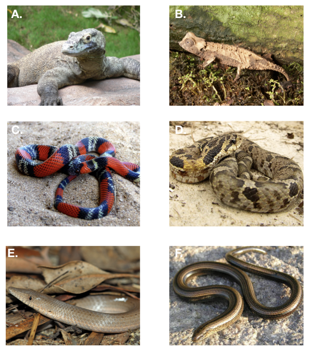
Figure 7.1. Squamates, legged and legless. A. Komodo dragon, B. Brookesia chameleon, C. False coral (Oxyrhopus guibei) and D. hognose snakes, E. a pygopodid - a limbless gecko and F. an anguid, another legless lizard. Photo credits: A: User:Raul654 / Wikimedia Commons / CC-BY-SA-3.0, B. Brian Gratwicke / CC-BY-2.0, C. User:Gionorossi / Wikimedia Commons / CC-BY-SA-4.0, D. User:Bladerunner8u / Wikimedia Commons / CC-BY-SA-3.0, E. User:Smacdonald / Wikimedia Commons / CC-BY-SA-2.5, F. User:Marek_bydg / Wikimedia Commons / CC-BY-SA-3.0.
Limblessness is an example of a discrete trait – a trait that can occupy one of a set of distinct character states. Analyzing the evolution of discrete traits requires a different modeling approach than what we used for continuous traits. In this chapter, I will discuss the Mk model (Lewis 2001), which is a general approach to modeling the evolution of discrete traits on trees. Fitting this model to comparative data will help us understand the evolution of traits like limblessness where species can be placed into one of a number of discrete character states.
Section 7.2: Modeling the evolution of discrete states
So far, we have only dealt with continuously varying characters. However, many characters of interest to biologists are best defined as characters with a set number of fixed states. For limblessness in squamates, each species is either legless (state 0) or not (state 1; actually, there are some species that might be considered “intermediate” Brandley et al. 2008, but we will ignore those for now). We might have particular questions about the evolution of limblessness in squamates. For example, how many times this character has changed in the evolutionary history of squamates? How often does limblessness evolve? Do limbs ever re-evolve? Is the evolution of limblessness related to some other aspect of the lives of these reptiles?
We will consider discrete characters where each species might exhibit one of k states. (In the limbless example above, k = 2). For characters with more than two states, there is a key distinction between ordered and unordered characters. Ordered characters can be placed in an order so that transitions only occur between adjacent states. For example, I might include “intermediate” species that are somewhere in between limbed and limbless – for example, the “mermaid skinks” (Sirenoscincus) from Madagascar, so called because they lack hind limbs (Figure 7.2, Moch and Senter 2011). An ordered model might only allow transitions between limbless and intermediate, and intermediate and limbed; it would be impossible under such a model to go directly from limbed to limbless without first becoming intermediate. For unordered characters, any state can change into any other state. In this chapter, I will focus mainly on unordered characters; we will return to ordered characters later in the book.
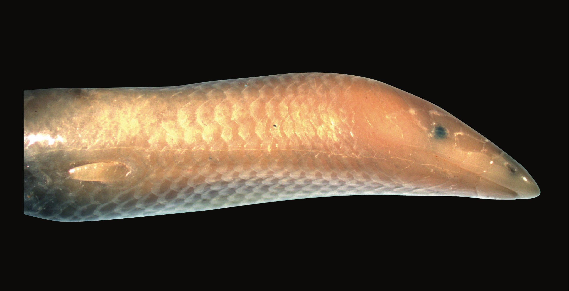
Figure 7.2. Mermaid skink, Aurélien Miralles / Wikimedia Commons CC-BY-SA-3.0.
Most work on the evolution of discrete characters on phylogenetic trees has focused on the evolution of gene or protein sequences. Gene sequences are made up of four character states (A, C, T, and G for DNA). Models of sequence evolution allow transitions among all of these states at certain rates, and may allow transition rates to vary across sites, among clades, or through time. There are a huge number of named models that have been applied to this problem (e.g. Jukes-Cantor, JC; General Time-Reversible, GTR; and many more, Yang 2006), and a battery of statistical approaches are available to fit these models to data (e.g. Posada 2008).
Any discrete character can be modeled in a similar way as gene sequences. When considering phenotypic characters, we should keep in mind two main differences from the analysis of DNA sequences. First, arbitrary discrete characters may have any number of states (beyond the four associated with DNA sequence data). Second, characters are typically analyzed independently rather than combining long sets of characters and assuming that they share the same model of change.
Section 7.3: The Mk Model
The most basic model for discrete character evolution is called the Mk model. First developed for trait data by Pagel (1994; although the name Mk comes from Lewis 2001). The Mk model is a direct analogue of the Jukes-Cantor (JC) model for sequence evolution. The model applies to a discrete character having k unordered states. Such a character might have k = 2, k = 3, or even more states. Evolution involves changing between these k states (Figure 7.3).
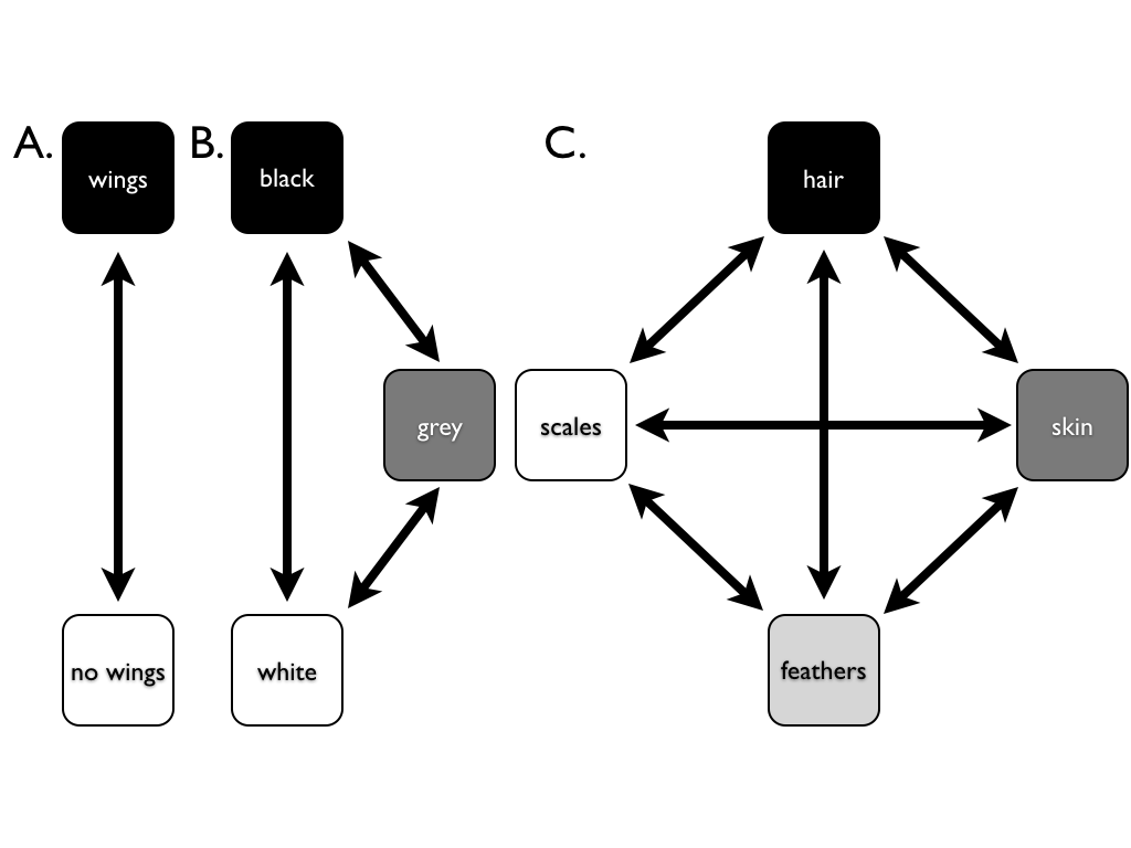
Figure 7.3. Examples of discrete characters with (A) k = 2, (B) k = 3, and (C) k = 4 states. Image by the author, can be reused under a CC-BY-4.0 license.
The basic version of the Mk model assumes that transitions among these states follow a Markov process. This means that the probability of changing from one state to another depends only on the current state, and not on what has come before. For example, it makes no difference if a lineage has just evolved the trait of “feathers,” or whether they have had feathers for millions of years – the probability of evolving a different character state is the same in both cases. The basic Mk model also assumes that every state is equally likely to change to any other state.
For the basic Mk model, we can denote the instantaneous rate of change between states using the parameter q. In general, qij is called the instantaneous rate between character states i and j. It is defined as the limit of the rate measured over very short time intervals1.
Again, for the basic Mk model, instantaneous rates between all pairs of characters are equal; that is, qij = qmn for all i ≠ j and m ≠ n.
We can summarize general Markov models for discrete characters using a transition rate matrix (Lewis 2001):
(eq. 7.1)
$$
\mathbf{Q} =
\begin{bmatrix}
-d_1 & q_{12} & \dots & q_{1k} \\
q_{21} & -d_2 & \dots & q_{2k} \\
\vdots & \vdots & \ddots & \vdots\\
q_{k1} & q{k2} & \dots & -d_k \\
\end{bmatrix}
$$
Note that the instantaneous rates are only entered into the off-diagonal parts of the matrix. Along the diagonal, these matrices always have a set of negative numbers. For any Q matrix, the sum of all the elements in each row is zero – a necessary condition for a transition rate matrix. Because of this, each negative number has a value, di, equal to the sum of all of the other numbers in the row. For example,
(eq. 7.2)
$$
d_1 = \sum_{i=2}^{k} q_{1i}
$$
For a two-state Mk model, k = 2 and rates are symmetric so that q12 = q21. In this case, we can write the transition rate matrix as:
(eq. 7.3)
$$
\mathbf{Q} =
\begin{bmatrix}
-q & q \\
q & -q \\
\end{bmatrix}
$$
Likewise, for k = 3, the transition rate matrix is:
(eq. 7.4)
$$
\mathbf{Q} =
\begin{bmatrix}
-2 q & q & q\\
q & -2 q & q\\
q & q & -2 q\\
\end{bmatrix}
$$
In general, the k-state transition matrix for a basic Mk model is:
(eq. 7.5)
$$
\mathbf{Q} =
\begin{bmatrix}
1-k & 1 & \dots & 1\\
1 & 1-k & \dots & 1\\
\vdots & \vdots & \ddots & \vdots\\
1 & 1 & \dots & 1\\
\end{bmatrix}
$$
Once we have this transition rate matrix, we can calculate the probability distribution of trait states after any time interval t using the equation (Lewis 2001):
(eq. 7.6)
P(t)=eQt
This equation looks simple, but calculating P(t) involves matrix exponentiation – raising e to a power defined by a matrix. This calculation is substantially different from raising e to the power defined by each element of a matrix2. The result is a matrix, P, of transition probabilities. Each element in this matrix (pij) gives the probability that starting in state i you will end up in state j over that time interval t. For the standard Mk model, there is a general solution to this equation:
(eq. 7.7)
$$
\begin{array}{l}
p_{ii}(t) = \frac{1}{k} + \frac{k-1}{k} e^{-kqt} \\
p_{ij}(t) = \frac{1}{k} - \frac{1}{k} e^{-kqt} \\
\end{array}
$$
In particular, when k = 2,
(eq. 7.8)
$$
\begin{array}{l}
p_{ii}(t) = \frac{1}{k} + \frac{k-1}{k} e^{-kqt} = \frac{1}{2} + \frac{2-1}{2}e^{-2qt}=\frac{1+e^{-2qt}}{2} \\
p_{ij}(t) = \frac{1}{k} - \frac{1}{k} e^{-kqt} = \frac{1}{2} - \frac{1}{2}e^{-2qt}=\frac{1-e^{-2qt}}{2} \\
\end{array}
$$
If we consider what happens when time gets very large in these equations, we see an interesting pattern. Any term that has e−t in it gets closer and closer to zero as t increases. Because of this, for all values of k, each pij(t) converges to a constant value, 1/k. This is the stationary distribution of character states, π, defined as the equilibrium frequency of character states if the process is run many times for a long enough time period. In general, the stationary distribution of an Mk model is:
(eq. 7.9)
$$
\pi =
\begin{bmatrix}
1/k & 1/k & \dots & 1/k\\
\end{bmatrix}
$$
In the case of k = 2,
(eq. 7.10)
$$
\pi =
\begin{bmatrix}
1/2 & 1/2 \\
\end{bmatrix}
$$
Section 7.4: The Extended Mk Model
The Mk model assumes that transitions among all possible character states occur at the same rate. However, that may not be a valid assumption. For example, it is often supposed that it is easier to lose a complex character than to gain one. We might want to fit models that allow for such asymmetries in rates.
For models of DNA sequence evolution there are a wide range of models allowing different rates between distinct types of nucleotides (Yang 2006). Unequal rates are usually incorporated into the Mk model in two ways. First, one can consider the symmetric model (SYM; Paradis et al. 2004). In the symmetric model, the rate of change between any two character states is the same forwards as it is backwards (that is, rates of change are symmetric; qij = qji). The rate for a particular pair of states might differ from other pairs of character states. Note that when k = 2 the symmetric model is identical to the basic Mk model. The rate matrix for this model has as many free rate parameters as there are pairs of character states:
(eq. 7.11)
$$
p = \frac{k(k-1)}{2}
$$
However, in general symmetric models will not have stationary distributions where all character states occur at equal frequencies, as noted above for the Mk model. We can account for these uneven frequencies by adding additional parameters to our model:
(eq. 7.12)
$$
\pi_{SYM} =
\begin{bmatrix}
\pi_1 & \pi_2 & \dots & 1 - \sum_{i=1}^{n-1} \pi_i
\end{bmatrix}
$$
Note that we only have to specify n − 1 equilibrium frequencies, since we know that they all sum to one. We have added n − 1 new parameters, for a total number of parameters:
(eq. 7.13)
$$
p = \frac{k(k-1)}{2} + n-1
$$
To obtain a Q-matrix for this model, we combine the information from both the relative transition rates and equilibrium frequencies:
(eq. 7.14)
$$
\mathbf{Q} =
\begin{bmatrix}
\cdot & r_1 & \dots & r_{n-1} \\
r_1 & \cdot & \dots & \vdots \\
\vdots & \vdots & \cdot & r_{k(k-1)/2} \\
r_{n-1} & \dots & r_{k(k-1)/2} & \cdot \\
\end{bmatrix}
\begin{bmatrix}
\pi_1 & 0 & 0 & 0 \\
0 & \pi_2 & 0 & 0 \\
0 & 0 & \ddots & 0 \\
0 & 0 & 0 & \pi_n \\
\end{bmatrix}
$$
In this equation I have left the diagonal of the first matrix as dots. The final Q-matrix must have all rows sum to one, so one can adjust the values of that matrix after the multiplication step.
In the case of a two-state model, for example, we can create a model where the forward rate is double the backward rate, and the equilibrium frequency of character one is 0.75. Then:
(eq. 7.15)
$$
\mathbf{Q} =
\begin{bmatrix}
\cdot & 1 \\
2 & \cdot \\
\end{bmatrix}
\begin{bmatrix}
0.75 & 0 \\
0 & 0.25 \\
\end{bmatrix}
=
\begin{bmatrix}
\cdot & 0.25 \\
1.5 & \cdot \\
\end{bmatrix}
=
\begin{bmatrix}
-0.25 & 0.25 \\
1.5 & -1.5 \\
\end{bmatrix}
$$
It is worth noting that this approach of setting parameters that define equilibrium state frequences, although borrowed from molecular evolution, is not completely standard in the comparative methods literature. One also sees equilibrium frequencies treated as a fixed property of the model, and assumed to be either equal across states or tied directly to the parameters in the Q-matrix.
The second common extension of the Mk model is called the all-rates-different model (ARD; Paradis et al. 2004). In this model every possible type of transition can have a different rate. There are thus k(k − 1) free rate parameters for this model, and again n − 1 parameters to specify the equilibrium frequencies of the character states.
The same algorithm can be used to calculate the likelihood for both of these extended Mk models (SYM and ARD). These models have more parameters than the standard Mk. To find maximum likelihood solutions, we must optimize the likelihood across the entire set of unknown parameters (see Chapter 7).
Section 7.5: Simulating the Mk model on a tree
We can also use the equations above to simulate evolution under an Mk or extended-Mk model on a tree (Felsenstein 2004). To do this, we simulate character evolution on each branch of the tree, starting at the root and progressing towards the tips. At speciation, we assume that both daughter species inherit the character state of their parental species immediately following speciation, and then evolve independently after that. At the end of the simulation, we will obtain a set of character states, one for each tip in the tree. The distribution of character states will depend on the shape of the phylogenetic tree (both its topology and branch lengths) along with the parameters of our model of character evolution.
We first draw a beginning character state at the root of the tree. There are several common ways to do this. For example, we can either draw from the stationary distribution or from one where each character state is equally likely. In the case of the standard Mk model, these are the same. For example, if we are simulating evolution under Mk with k = 2, then state 0 and 1 each have a probability of 1/2 at the root. We can draw the root state from a binomial distribution with pstate0 = 0.5.
Once we have a character state for the root, we then simulate evolution along each branch in the tree. We start with the (usually two) branches descending from the root. We then proceed up the tree, branch by branch, until we get to the tips.
We can understand this algorithm perfectly well by thinking about what happens on each branch of the tree, and then extending that algorithm to all of the branches (as described above). For each branch, we first calculate P(t), the transition probability matrix, given the length of the branch and our model of evolution as summarized by Q and the branch length t. We then focus on the row of P(t) that corresponds to the character state at the beginning of the branch. For example, let’s consider a basic two-state Mk model with q = 0.5. We will call the states 0 and 1. We can calculate P(t) for a branch with length t = 3 as:
(eq. 7.16)
$$
\mathbf{P}(t) = e^{\mathbf{Q} t} = exp(
\begin{bmatrix}
-0.5 & 0.5 \\
0.5 & -0.5 \\
\end{bmatrix}
\cdot 3) =
\begin{bmatrix}
0.525 & 0.475 \\
0.475 & 0.525 \\
\end{bmatrix}
$$
If we had started with character state 0 at the beginning of this branch, we would focus on the first row of this matrix. We want to end up at state 0 with probability 0.525 and change to state 1 with probability 0.475. We again draw a uniform random deviate u, and choose state 0 if 0 ≤ u < 0.525 and state 1 if 0.525 ≤ u < 1. If we started with a different character state, we would use a different row in the matrix. If this is an internal branch in the tree, then both daughter species inherit the character state that we chose immediately following speciation – but might diverge soon after! By repeating this along every branch in the tree, we obtain a set of character states at the tips of the tree. This is then the output of our simulation.
Two additional details here are worth noting. First, the procedure for simulating characters under the extended-Mk model are identical to those above, except that the calculation of matrix exponentials is more complicated than in the standard Mk model. Second, if you are simulating a character with more than two states, then the procedure for drawing a random number is slightly different3.
We can apply this approach to simulate the evolution of limblessness in squamates. Below, I present the results of three such simulations. These simulations are a little different than what I describe above because they consider all changes in the tree, rather than just character states at nodes and tips; but the model (and the principal) is the same. You can see that the model leaves an imprint on the pattern of changes in the tree, and you can imagine that one might be able to reconstruct the model using a phylogenetic comparative approach. Of course, typically we know only the tip states, and have to reconstruct changes along branches in the tree. We will discuss parameter estimation for the Mk and extended-Mk models in the next chapter.
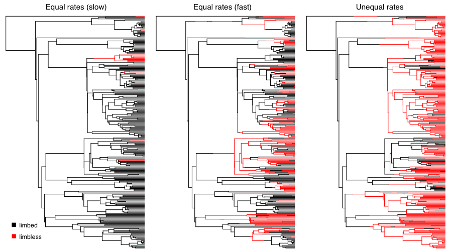
Figure 7.4. Simulated character evolution on a phylogenetic tree of squamates (from Brandley et al. 2008) under an equal-rates Mk model with slow, fast, and asymmetric transition rates (from right to left). In all three cases, I assumed that the ancestor of squamates had limbs. Image by the author, can be reused under a CC-BY-4.0 license.
Section 7.6: Chapter summary
In this chapter I have described the Mk model, which can be used to describe the evolution of discrete characters that have a set number of fixed states. We can also elaborate on the Mk model to allow more complex models of discrete character evolution (the extended-Mk model). These models can all be used to simulate the evolution of discrete characters on trees.
In summary, the Mk and extended Mk model are general models that one can use for the evolution of discrete characters. In the next chapter, I will show how to fit these models to data and use them to test evolutionary hypotheses.
Section 7.7: Footnotes
1: Imagine that you calculate a rate of character change by counting the number of changes of state of a character over some time interval, t. You can calculate the rate of change as nchanges/t. The instantaneous rate is the value that this rate approaches as t gets smaller and smaller so that the time interval is nearly zero.
2: I will not cover the details of matrix exponentiation here – interested readers should see Yang (2006) for details – but the calculations are not trivial.
3: One still obtains the relevant row from P(t) and draws a uniform random deviate u. Imagine that we have a ten-state character with states 0 - 9. We start at state 0 at the beginning of the simulation. Again using q = 0.5 and t = 3, we find that:
(eq. 7.17)
$$
\begin{array}{l}
p_{ii}(t) = \frac{1}{k} + \frac{k-1}{k} e^{-kqt} = \frac{1}{10}+\frac{9}{10}e^{-2 \cdot 0.5 \cdot 3} = 0.145\\
p_{ij}(t) = \frac{1}{k} - \frac{1}{k} e^{-kqt} \frac{1}{10} - \frac{1}{10}e^{-2 \cdot 0.5 \cdot 3} = 0.095\\
\end{array}
$$
We focus on the first row of P(t), which has elements:
$$
\begin{bmatrix}
0.145 & 0.095 & 0.095 & 0.095 & 0.095 & 0.095 & 0.095 & 0.095 & 0.095 & 0.095 \\
\end{bmatrix}
$$
We calculate the cumulative sum of these elements, adding them together so that each number represents the sum of itself and all preceding elements in the vector:
$$
\begin{bmatrix}
0.145 & 0.240 & 0.335 & 0.430 & 0.525 & 0.620 & 0.715 & 0.810 & 0.905 & 1.000 \\
\end{bmatrix}
$$
Now we compare u to the numbers in this cumulative sum vector. We select the smallest element that is still strictly larger than u, and assign this character state for the end of the branch. For example, if u = 0.475, the 5th element, 0.525, is the smallest number that is still greater than u. This corresponds to character state 4, which we assign to the end of the branch. This last procedure is a numerical trick. Imagine that we have a line segment with length 1. The cumulative sum vector breaks the unit line into segments, each of which is exactly as long as the probability of each event in the set. One then just draws a random number between 0 and 1 using a uniform distribution. The segment that contains this random number is our event.
References
Brandley, M. C., J. P. Huelsenbeck, and J. J. Wiens. 2008. Rates and patterns in the evolution of snake-like body form in squamate reptiles: Evidence for repeated re-evolution of lost digits and long-term persistence of intermediate body forms. Evolution. Wiley Online Library.
Felsenstein, J. 2004. Inferring phylogenies. Sinauer Associates, Inc., Sunderland, MA.
Hedges, S. B., J. Dudley, and S. Kumar. 2006. TimeTree: A public knowledge-base of divergence times among organisms. Bioinformatics 22:2971–2972.
Lewis, P. O. 2001. A likelihood approach to estimating phylogeny from discrete morphological character data. Syst. Biol. 50:913–925.
Moch, J. G., and P. Senter. 2011. Vestigial structures in the appendicular skeletons of eight African skink species (squamata, scincidae). J. Zool. 285:274–280. Blackwell Publishing Ltd.
Pagel, M. 1994. Detecting correlated evolution on phylogenies: A general method for the comparative analysis of discrete characters. Proc. R. Soc. Lond. B Biol. Sci. 255:37–45. The Royal Society.
Paradis, E., J. Claude, and K. Strimmer. 2004. APE: Analyses of phylogenetics and evolution in R language. Bioinformatics 20:289–290. academic.oup.com.
Pianka, E. R., L. J. Vitt, N. Pelegrin, D. B. Fitzgerald, and K. O. Winemiller. 2017. Toward a periodic table of niches, or exploring the lizard niche hypervolume. Am. Nat. 190:601–616. journals.uchicago.edu.
Posada, D. 2008. jModelTest: Phylogenetic model averaging. Mol. Biol. Evol. 25:1253–1256. academic.oup.com.
Streicher, J. W., and J. J. Wiens. 2017. Phylogenomic analyses of more than 4000 nuclear loci resolve the origin of snakes among lizard families. Biol. Lett. 13. rsbl.royalsocietypublishing.org.
Vitt, L. J., E. R. Pianka, W. E. Cooper Jr, and K. Schwenk. 2003. History and the global ecology of squamate reptiles. Am. Nat. 162:44–60. journals.uchicago.edu.
Yang, Z. 2006. Computational molecular evolution. Oxford University Press.